Theoretical Background
December 14, 2016 12:13 pmHeisenberg’s uncertainty principle is probably the most famous statement of modern physics and familiar to most in the formulation of standard deviations, such as for position and momentum , or as , for arbitrary non-commuting observables and . However, a naive Heisenberg-type error-disturbance relation (EDR), for non-commuting observables, denoted as is not valid in general. In addition, if one looks closely at the way the uncertainty principle is used by Heisenberg and Bohr in their analysis of though experiments, it emerges that their arguments cannot be – and in fact are not – based on a relation in terms of standard deviations. The uncertainty principle turns out to be a much more intricate statement.
Contents:
Heisenberg’s Uncertainty Principle
Measurement Uncertainty Relations
””””Ozawa’s generalized Uncertainty Relation
””””””””Tighter uncertainty relations
””””””””Mixed state uncertainty relations
””””Busch/Werner/Lahti’s Proof of Heisenberg’s original Error-Disturbance Relation
””””Information-theoretic (entropic) Uncertainty Relations
””””””””Entropic uncertainty relations for projective qubit measurements
””””””””Information-theoretic uncertainty relations for general qubit measurements
Preparation Uncertainty Relations
””””Tight State-Independent Uncertainty Relations for Qubits
””””Entropic Overlap Uncertainty Relations
S
Heisenberg’s Uncertainty Principle
The uncertainty principle represents, without any doubt, one of the most important cornerstones of the Copenhagen interpretation of quantum theory. In his celebrated paper from 1927 1 Werner Heisenberg 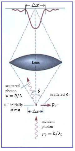 gives at least three distinct statements about the limitations on preparation and measurement of physical systems: (i) It is impossible to prepare a system such that a pair of noncommuting (incompatible) observables are arbitrarily well defined. In the original paper the observables are represented by position and momentum. In every state the probability distributions of the observables will have widths that obey a (preparation) uncertainty relation. (ii) Incompatible observables cannot be jointly measured – or more precisely simultaneously, with arbitrary accuracy. What can be done is to perform approximate joint measurements with inaccuracies that satisfy an uncertainty relation or inaccuracy relations “Ungenauigkeitsrelationen“, which was Heisenberg’s favorite terminology. (iii) it is not possible to measure an observable without disturbing a subsequent measurement of an (incompatible) observable and vice versa. The inaccuracy (error) of the measurement of the first and the disturbance of the measurement of the second observable obey an error-disturbance uncertainty relation. Heisenberg illustrates this in his paper by proposing a reciprocal relation for mean error “mittlere Fehler“ and disturbance of a measurement using the famous – ray microscope thought experiment: “At the instant when the position is determined—therefore, at the moment when the photon is scattered by the electron—the electron undergoes a discontinuous change in momentum. is change is the greater the smaller the wavelength of the light employed— that is, the more exact the determination of the position . . .” 1. Heisenberg follows Einstein’s realistic view, that is, to base a new physical theory only on observable quantities (elements of reality), arguing that terms like velocity or position make no sense without defining an appropriate apparatus for a measurement. By solely considering the Compton effect, named after the American physicist Arthur Holly Compton Heisenberg gives a rather heuristic estimate for the product of the inaccuracy (error) of a position measurement and the disturbance induced on the particles momentum, denoted by . This equation can be referred to as a measurement uncertainty (i) or as an error-disturbance uncertainty relation (EDR). Heisenberg’s original formulation can be read in modern treatment as for error of a measurement of the position observable and disturbance of the momentum observable induced by the position measurement. Just as a side node: Heisenberg himself never used the term “principle” for his relations, as already stated above he referred to them as inaccuracy relations “Ungenauigkeitsrelationen” or indeterminacy relations “Unbestimmtheitsrelationen“.
However, most modern textbooks introduce the uncertainty relation in terms of a preparation uncertainty (ii) relation denoted by , originally proved by Earle Hesse Kennard 2 for the standard deviations and and 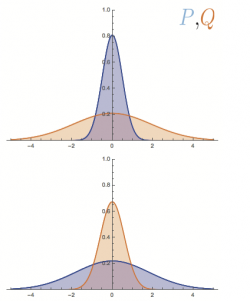 of the position observable and the momentum observable in an arbitrary state , where the standard deviation is defined by . This formulation of the uncertainty principle is uncontroversial and has been tested with several quantum systems including neutrons. However it does not capture Heisenberg’s initial intensions: Kennard’s formulation is an inequality for statistical distributions of not a joint but rather single measurements of either or . It is an intrinsic uncertainty inherent to any quantum system independent whether it is measured or not. The unavoidable recoil caused by the measuring device is ignored here. The reciprocal behavior of the distributions of and is illustrated on the right side. Heisenberg actually derived Kennard’s relation, from above, for Gaussian wave functions , applied this relation to the state just after the measurement with error and disturbance , and concluded his relation from the additional, implicit assumptions and . However, his assumption holds only for a restricted class of measurements and holds if the initial state is the momentum eigenstate state, but it does not hold generally. In 1929, Howard Percy “Bob” Robertson 3 extended Kennard’s relation () to an arbitrary pair of observables and as , with the commutator . The corresponding generalized form of Heisenberg’s original error-disturbance uncertainty relation would read . But the validity of this relation is known to be limited to specific circumstances.
Types of Uncertainty Relations
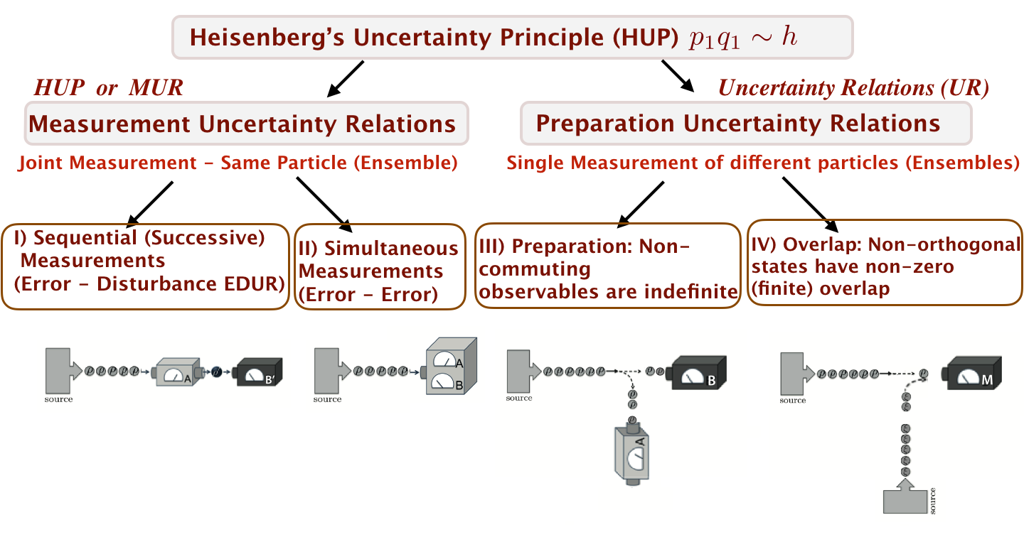
I) & II) Measurement Uncertainty: A measurement of one observable necessarily “disturbs” other observables – either in a sequential or simultaneous measurement.
III) Preparation Uncertainty: The quantum description of a physical system cannot simultaneously assign definite (sharp) values to all observables.
IV) Overlap Uncertainty: Different physical states cannot in general be unambiguously distinguished by measurement.
II)S
Measurement Uncertainty Relations
Ozawa’s generalized Uncertainty Relation
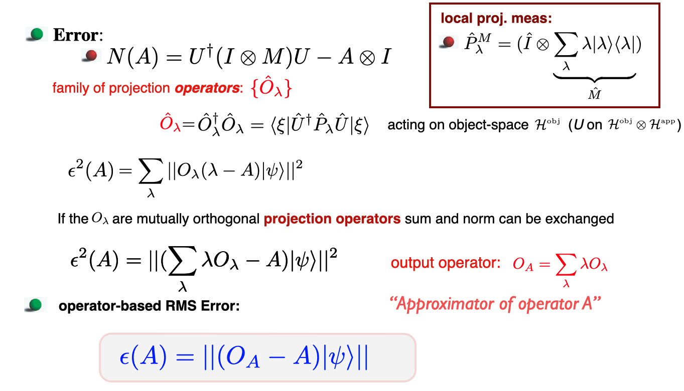
In the year 2003 Japanese theoretical physicist Masanao Ozawa proposed a new error- disturbance uncertainty relation 4, and proved its universal validity in the general theory of quantum measurements (see here for details of the derivation). Here denotes the root-mean-square (r.m.s.) 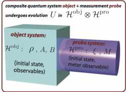 error of anarbitrary measurement for an observable , is the r.m.s. disturbance on another observable induced by the measurement, and and are the standard deviations of and in the state before the measurement. Here error and disturbance are defined via an indirect measurement model for an apparatus A measuring an observable of an object system S as and . Here is the initial state of system S, which is associated with Hilbert space . is the state of the probe system P before the measurement, defined on Hilbert space , and an observable , referred to as meter observable of P. The time evolution of the composite system P+S during the measurement interaction is described by a unitary operator on . The Hilbert–Schmidt norm is used where the norm of a state vector in Hilbert space is given by the square root of its inner product: . A schematic illustration of a measurement apparatus A is given aside. In the general case, where a local projective measurement of the probe system generates a POVM the error yields:
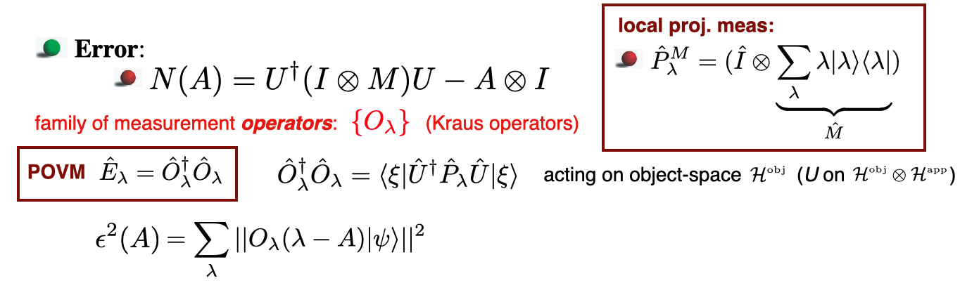
For projective measurements this simplifies to
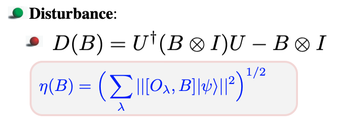
For the disturbance we get
See here for our experimental test of Ozawa’s generalized error-disturbance uncertainty relation.
Tighter uncertainty relations
Though universally valid Ozawa’s relation from above is not optimal. The reason for this is that three terms in Ozawa’s relation come from three 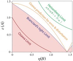 independent uses of Robertson’s relation (see here for details) to different pairs of observables. Although this indeed leads to a valid relation, this is not optimal because the three Robertson’s relations – and consequently Ozawa’s relation – generally cannot be saturated simultaneously. Thus, Cyril Branciard 6 showed that one can improve on the sub-optimality of Ozawa’s proof and derived the following trade-off relation between error and disturbance by applying two geometric lemmas:
 ![]() , where we have again . For the special case , which implies , and replacing and by and , respectively, the above equation can be strengthened yielding the tight relation
, where we have again . For the special case , which implies , and replacing and by and , respectively, the above equation can be strengthened yielding the tight relation ![]() , as illustrated aside in comparison with Heisenberg’s and Ozawa’s error-disturbance uncertainty relations. Click here for our experimental test of a tight error-disturbance uncertainty relation.
, as illustrated aside in comparison with Heisenberg’s and Ozawa’s error-disturbance uncertainty relations. Click here for our experimental test of a tight error-disturbance uncertainty relation.
Mixed state uncertainty relations
Aiming in of an improvement of error-disturbance uncertainty relations (EDUR) a stronger inequality was proposed. Later, it was pointed out that the relation above is not stringent for mixed states in general, when the Robertson bound is simply extended to , which decreases for mixed states and vanishes for totally mixed states. Further improvement of the bound was put forward by Masanao Ozawa who could show that the constant can be replaced by a stronger constant defined by . This new parameter coincides with the Robertson bound when is a pure state, but makes the EDUR stronger for a mixed ensemble. Our experimental test for mixed state uncertainty relations is reported here.
Busch/Werner/Lahti’s Proof of Heisenberg’s original Error-Disturbance Relation
In 2013, as a result of various attempts of rigorous reformulations of Heisenberg’s original Error-Disturbance Relation, Paul Busch, and Pekka Lahti, and Reinhard F. Werner (BLW) provided a general, quantitative quantum version of Heisenberg’s original semiclassical uncertainty, by applying appropriate definitions of our and disturbance 7 . Unlike in Ozawa’s approach, where the measurement process is described by the interaction of a quantum object with a probe, in BLW’s scheme error and disturbance are evaluated from the difference between output probability distributions, as illustrated schematically below. This is achieved by performing highly accurate single measurements, so-called reference or control measurements of the (general) target observ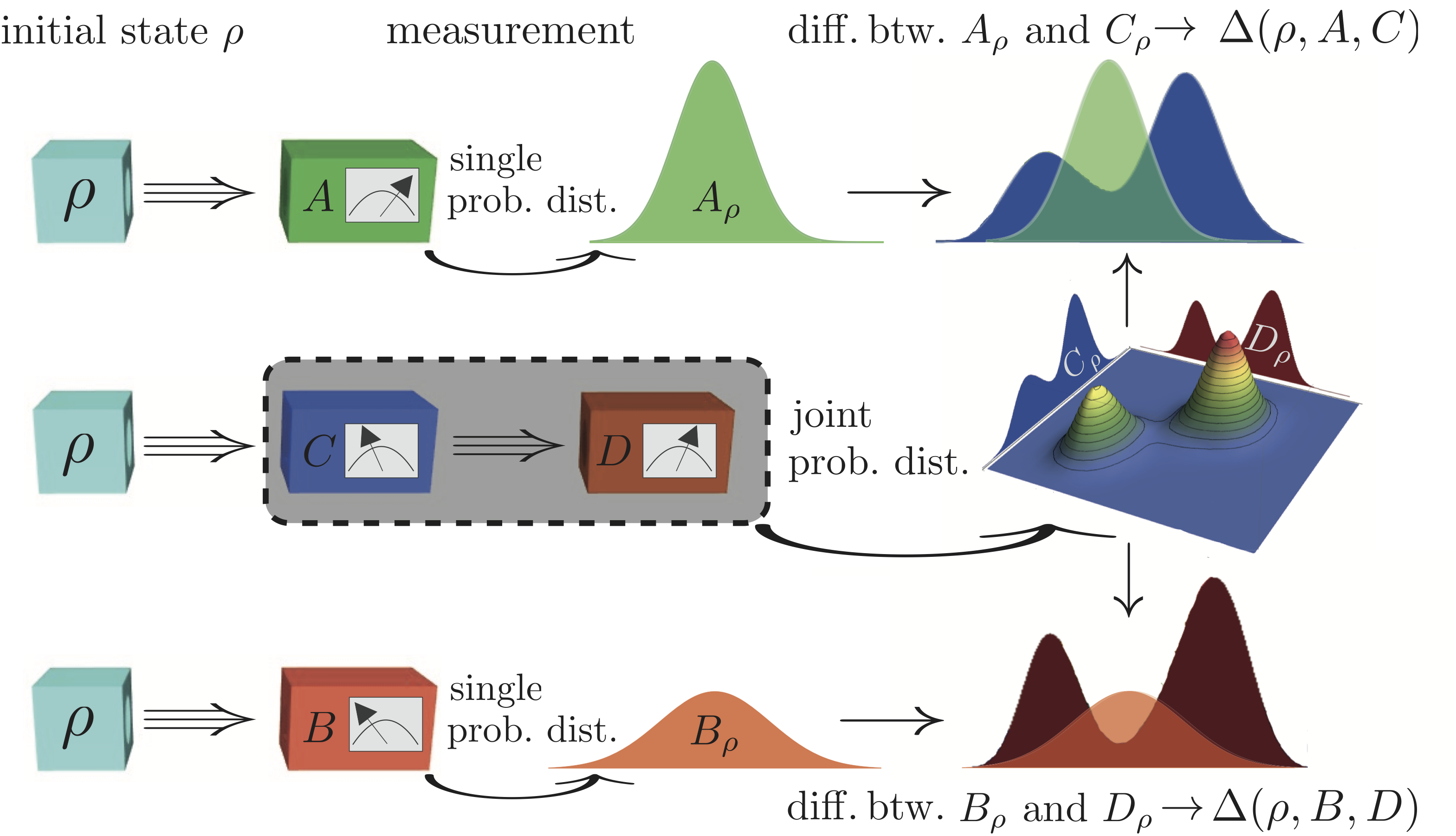 ables and in the input state , yielding probability distributions and . In a next step, using a successive measurement scheme, the observable is approximated by an observable , thereby inducing a change of the input state and thus a modification of the subsequent -measurement to be effectively a measurement of an observable on . The marginal distributions and of the joint probability distribution obtained from the successive measurement are then compared with the output statistics of the reference (single) measurements. Hence, the difference between and then account for the state dependent error, denoted as . Likewise the difference between and is the state dependent disturbance, which is expressed as . Both quantities are evaluated using the Wasserstein-2-distance resulting in for error and for disturbance. For the special case of position and momentum Heisenberg’s original error-disturbance relation is maintained in terms of , where and are the marginal observables of some joint measurement device. However for qubit observables the respective inequality is given by , where the bound accounts for the incompatibility of and 8 . See here for our experimental comparison between the theoretical approaches of BWL with Ozawa’s.
Information-theoretic (entropic) Uncertainty Relations
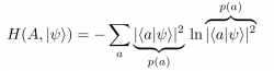
The uncertainty relation, as formulated by Robertson Relation in terms of standard deviations has two flaws, which was first recognized by Israeli-born British physicist David Deutsch in 1983 9 : i) standard deviation not optimal measure for all states, there exist certain states, for which the standard deviation diverges (see here for an example). ii) the boundary (right hand side of any uncertainty relation) can become zero for non-commuting observables (this is also the case for our neutron spins for a combination of and ). So Deutsch suggested to seek a theorem of linear algebra in the form . Heisenberg’s (Kaennard) inequality has that form but its generalization does not. In order to represent a quantitative physical notion of “uncertainty, must at least possess the following elementary property: If and only if is a simultaneous eigenstate of and may become zero. From this we can infer a property of , namely that it must vanish if and only if and have an eigenstate in common. “The most natural measure of the uncertainty in the result of a measurement or preparation of a single discrete observable is the (Shannon) entropy 9 ” (see here for a short introduction to probability theory). According to Claude Shannon entropy is the expected (average) information received, which consists of the so called self-information a.k.a. surprisal and its probability to occur defined as

which can be expressed in the language of quantum mechanics as
Information-theoretic uncertainty relations for projective qubit measurements (dichotomic case)
A tight noise-disturbance uncertainty relation for projective qubit measurements, with two possible outcames, i.e., dichotomic, including appropriate information-theoretic definitions for noise and disturbance in quantum measurements were proposed in 10. The procedure is the following: Randomly selected eigenstates of and , with and , are sent into a measurement apparatus , followed by a correction operation . The experimental procedure is schematically illustrated below:
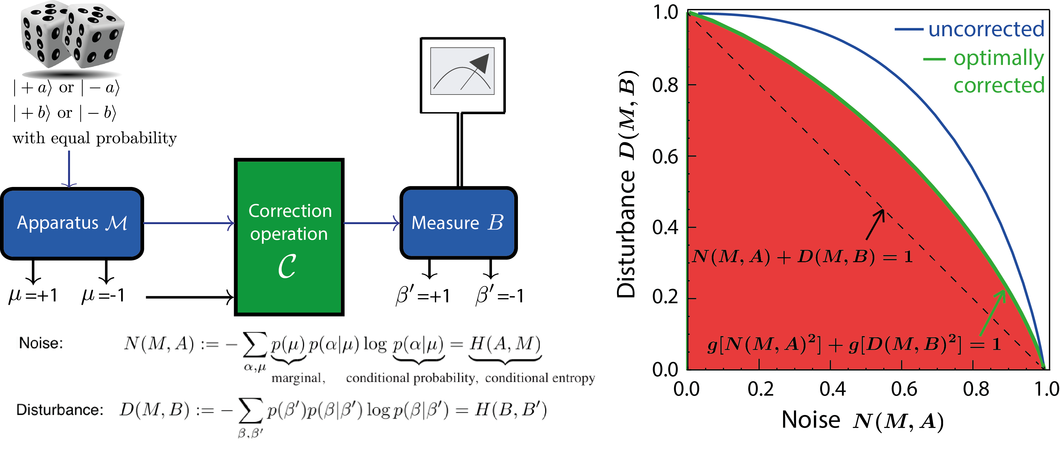
From the obtained data a state independent noise-disturbance trade-off relation in terms of , with , is inferred. The predicted values are given by the blue line in the plot above (right). For maximally incompatible qubit observables, represented by the Pauli matrices and we have been able to significantly strengthen this relation to the tight relation , where denotes the inverse of the function given by . Experimentally this is achieved by applying a correction operation after the measurement yielding the green curve in the above diagram. For projective measurements theoretic predictions for noise and disturbance are given by and , respectively. See here for our experimental test of a tight entropic noise-disturbance uncertainty relations for projective qubit measurements.
Information-theoretic uncertainty relations for general qubit measurements (POVM case)
A tight information-theoretic (or entropic) uncertainty relation for general qubit measurements, that is a positive-operator valued measure (POVM), was proposed recently by Alastair A. Abbott and Cyril Branciard in 11, discussing both, entropic noise-noise and entropic noise-disturbance uncertainty relations (see here for details on POVMs).
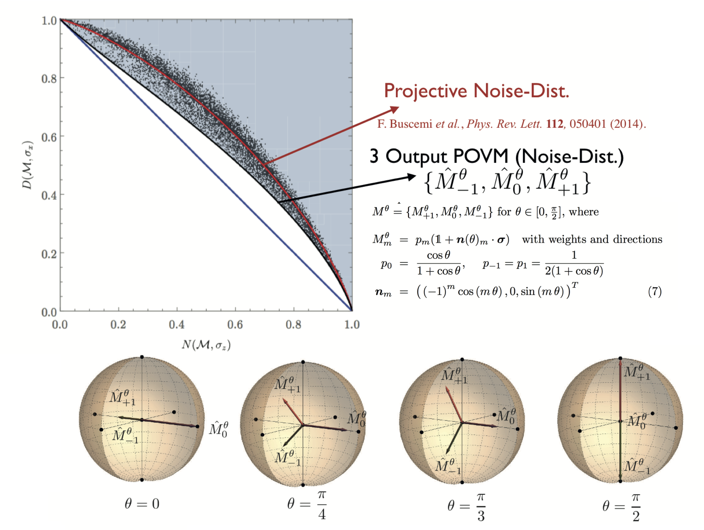
In the case of this particular three-outcome POVM theoretic predictions for noise and disturbance are given by and , respectively. See here for our experimental test of a tight entropic noise-disturbance uncertainty relations for POVM qubit measurements.
SPreparation Uncertainty Relations
In his seminal paper from m 1927 1 Heisenberg did not give a rigorous mathematical formulation uncertainty principle bit rather a heuristic description, giving the uncertainty principle a rather qualitative character. However, a short time after Heisenberg’s vague presentation an inequality holding for arbitrary states was proven by by Kennard 2 expressed as , in terms of standard deviations and and of the position observable and the momentum observable in an arbitrary state , where the standard deviation is defined by . Soon later, in 1929, Robertson 3 extended Kennard’s relation to an arbitrary pair of observables and as with the commutator . However, Robertson uncertainty relation follows from a slightly stronger inequality namely the Schrödinger uncertainty relation 12 which is given by , where we have 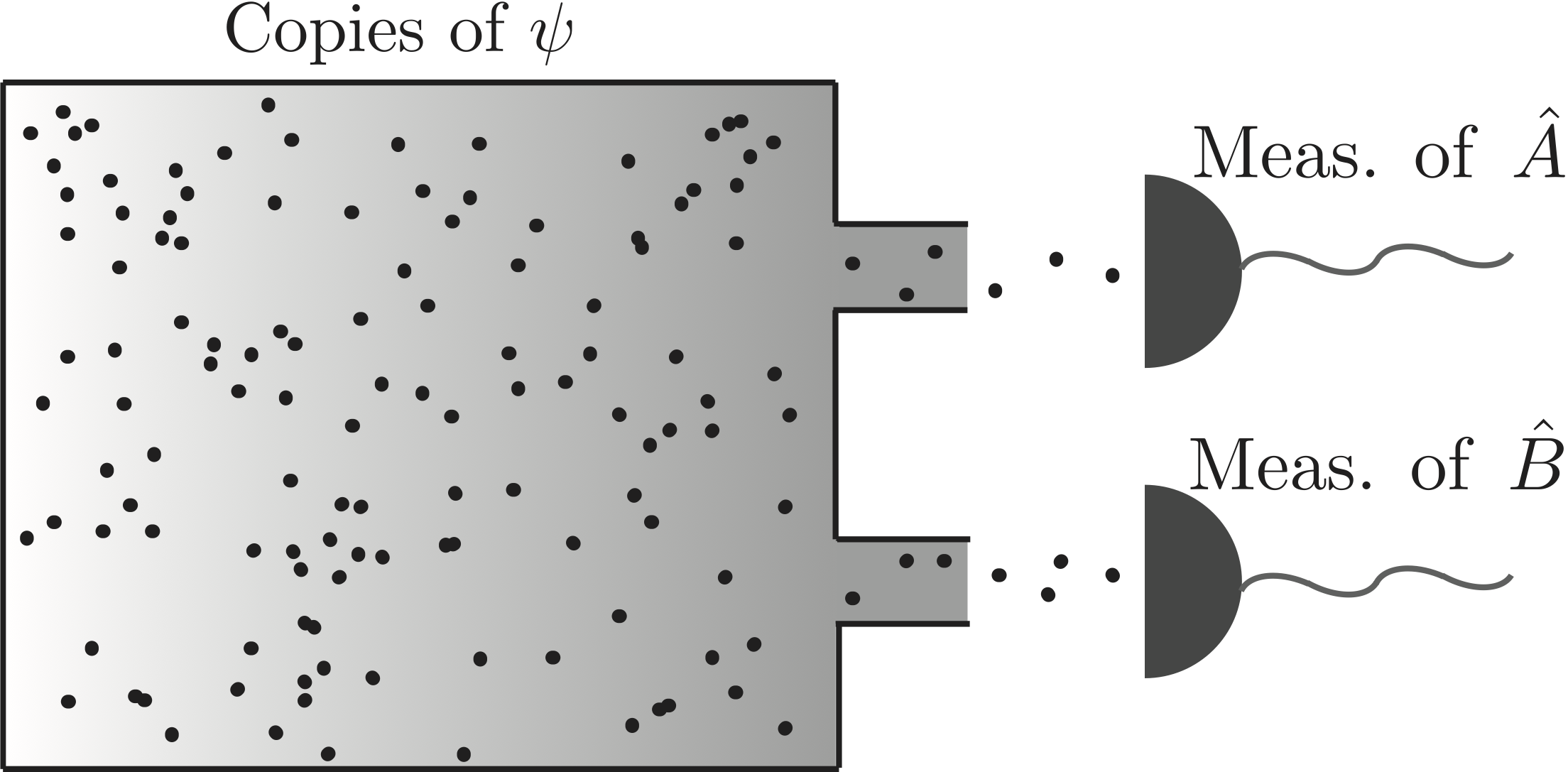 introduced the anticommutator . The standard deviations characterize the dispersion of a distribution and are a measure for the spreading of a set of values around the mean value. This means that the inequalities just described are of statistical nature and therefore do not describe the systematic imperfections of a quantum measurement scheme, as originally proposed by Heisenberg. This, in particular, implies an error-free measurement. The standard deviation attained by (ideally infinite) repetitions of the measurement on exactly identical states . Physically, one should associate preparation uncertainty relations with a reservoir of particles which contains a large number of copies of one and the same state as illustrated aside. If we have particles particles are exposed to a measurement of observable and particles are used for the measurement of observable . From the obtained count rates we can calculate the the standard deviations of the output distributions for the observables and , which are required for the preparation uncertainty relation for the observables and .
Tight State-Independent Uncertainty Relations for Qubits
The well-known Robertson–Schrödinger uncertainty relation has state-dependent lower bounds, which are trivial for certain states. Therefore C. Branciard and co-workers proposed a general approach to deriving tight state-independent uncertainty relations for qubit measurements that completely characterize the obtainable uncertainty values in 13. Their relations can be transformed into equivalent tight entropic uncertainty relations, or more generally in terms of any measure of uncertainty that can be written as a function of the expectation value. For any pair of Pauli observables and , with every quantum state satisfies the condition , which is illustrated below for left and right. The values () on its boundary saturate the relation from above. The concentric circles [ellipses] represent the regions of permitted values for mixed states with bounded Bloch vector norms , while the outer blue circle [ellipse] represents the expectation values of pure states.
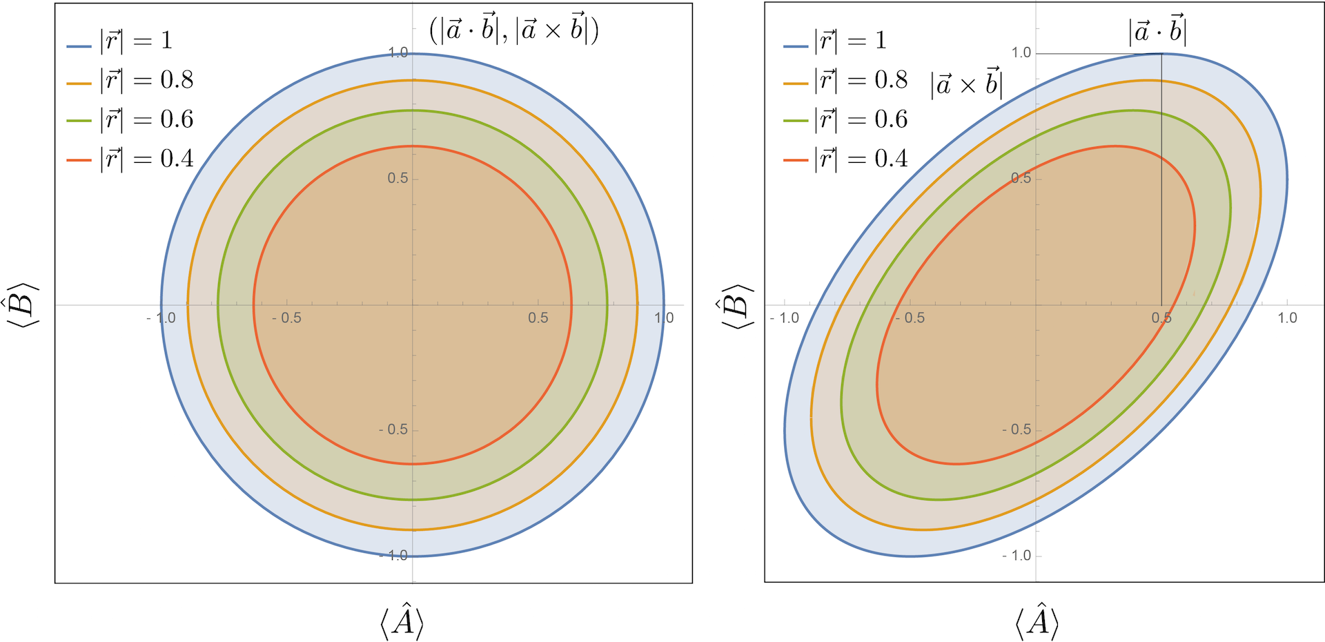
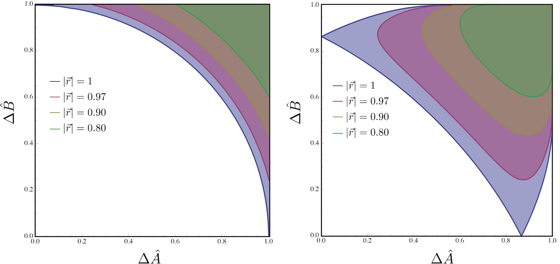
The standard deviation and expectation value are connected via and , since every Pauli operator satisfies . Hence, the tight state-independent uncertainty relations from above can be rewritten in terms of standard deviations as , which is illustrated below for (the color-coding has changed due to different values of ).
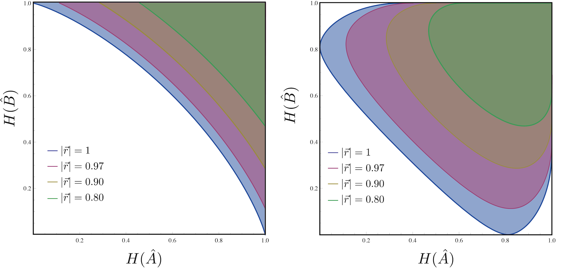
In the case of qubits, the Shannon entropy of a Pauli observable can be directly expressed in terms of the expectation value , namely: , where is the binary entropy function defined as , or with , where denotes the inverse function of . Then one obtains the following tight relation for two Pauli observables , which is illustrated below (again) for (the color-coding has changed due to different values of ).
Finally, it should be noted here, that it is also possible to go beyond projective measurements and give similar relations for positive-operator valued measures (POVMs) for qubits with binary outcomes.
Entropic Overlap Uncertainty Relations
The qubit preparation uncertainty region , for two observables and (), can be completely characterized by the tight preparation uncertainty relation in terms of standard deviations as . An equivalent formulation in terms of entropies reads . Interestingly, the region is nonconvex for and convex for . Hence, for the above relation expresses the tight uncertainty relation .
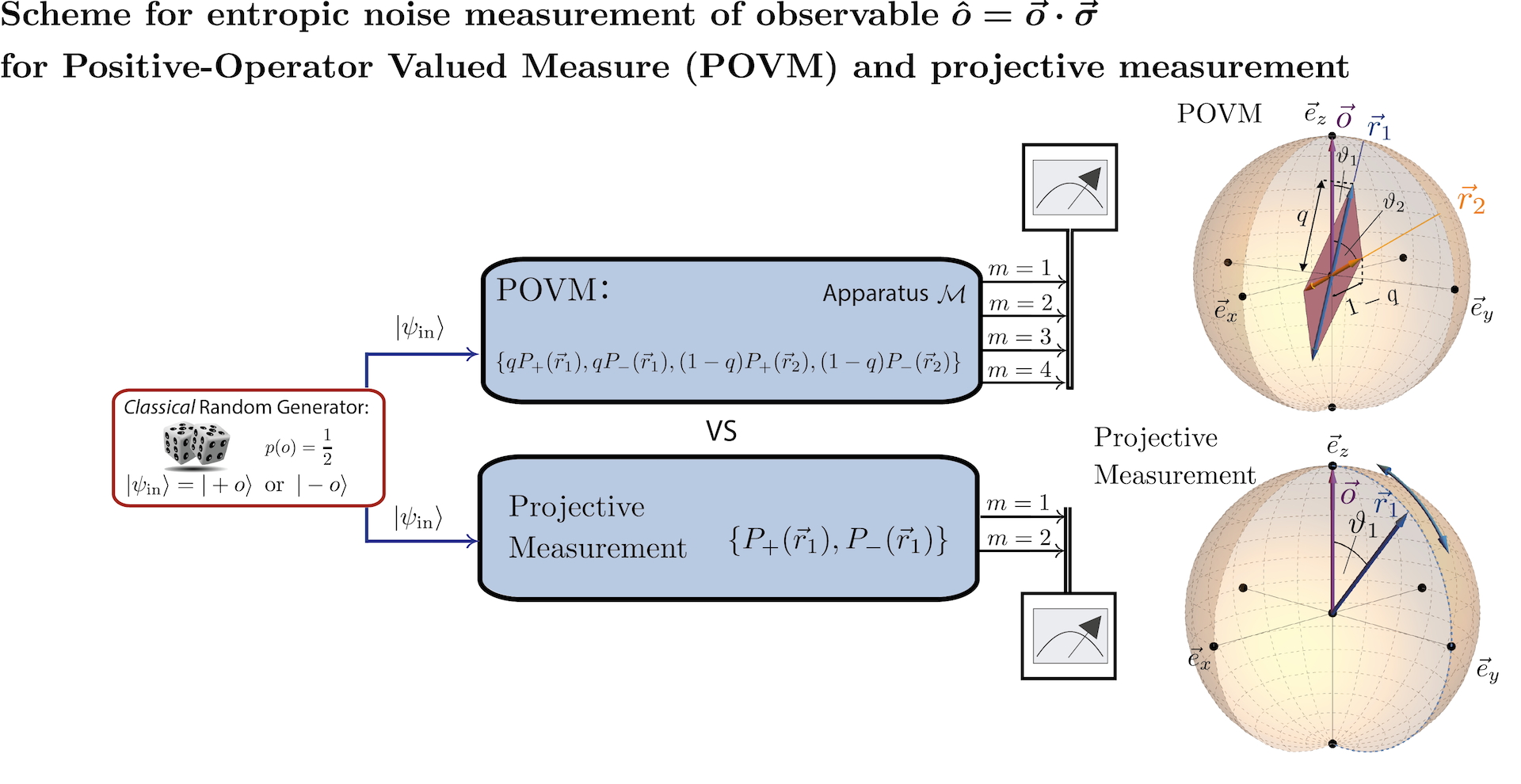
For no analytic form for the convex hull of exists in general. However, for , i.e., for orthogonal Pauli measurements for instance as and , the relation can be given explicitly and we have the simple tight relation . Then an apparatus implementing the POVM , which performs a combination of these two projective measurements with probabilities and , respectively, allows for may reach any point in the region and is therefore able to saturate the boundary, which is illustrated aside for the noise of an qubit observable .
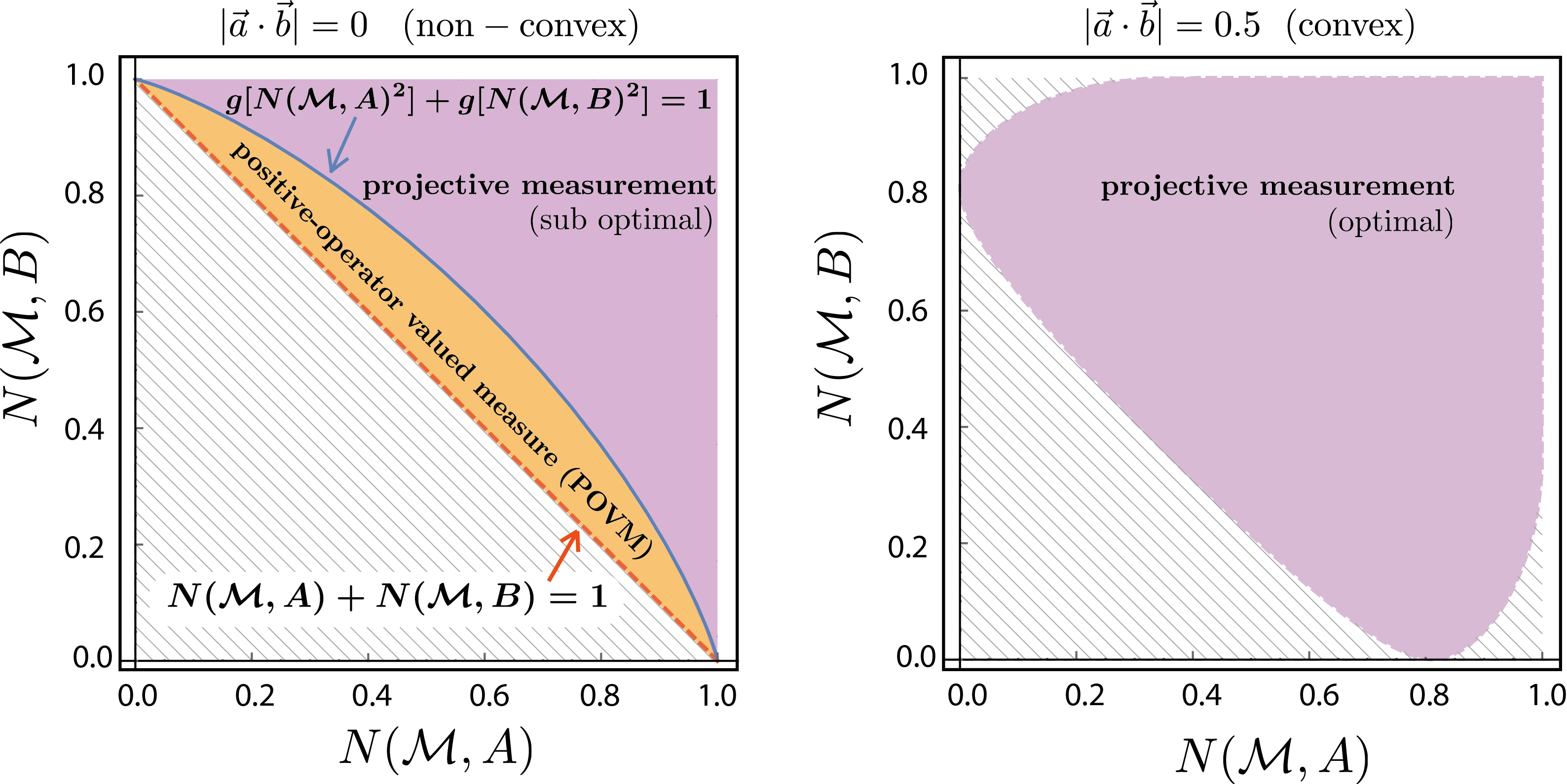
Hence, projective measurements are able to saturate the tradeoff when is convex, but are suboptimal when it is not, i.e., non-convex. Above on the left you can see the expected results for a noise-noise Plot for and meaning and on the right side. See here for our experimental test of entropic overlap uncertainty relations.
1. W. Heisenberg, Z. Phys. 43, 172 (1927). ↩
2. E. H. Kennard, Z. Phys. 44, 326 (1927). ↩
3. H. P. Robertson, Phys. Rev. 34, 163 (1929). ↩
4. M. Ozawa, Phys. Rev. A 67, 042105 (2003). ↩
6. C. Branciard, Proc. Natl. Acad. Sci. USA 17, 6742-6747 (2013). ↩
7. P. Busch, P. Lahti, and R. F. Werner Phys. Rev. Lett. 17, 6742-6747 (2013). ↩
8. P. Busch, P. Lahti, and R. F. Werner Phys. Rev. A 89, 012129 (2014). ↩
9. D. Deutsch, Phys. Rev. Lett. 50, 631 (1983). ↩
10. F. Buscemi, M. J. W. Hall, M. Ozawa, and M. M. Wilde, Phys. Rev. A 112, 050401 (2014). ↩
11. A. A. Abbott and C. Branciard, Phys. Rev. A 94, 062110 (2016). ↩
12. E. Schrödinger, Sitzungsberichte der Preussischen Akademie der Wissenschaften, Physikalisch-mathematische Klasse 14, 296–303 (1930). ↩
13. A. A. Abbott P-L Alzieu, M. J. W. Hall and C. Branciard, Mathematics 4, 8 (2016). ↩