Probability Theory
July 26, 2017 11:16 amProbability theory is the branch of mathematics concerned with probability, in other words it is the study of uncertainty. The mathematical theory of probability is highly sophisticated, and delves into a branch of analysis which is also known as measure theory.
Contents:
Basic Concept of Probability Theory
Joint & Conditional Probabilities
Self-Information & Entropy
Basic Concept of Probability Theory
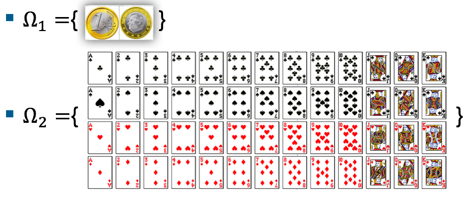
In order to define a probability on a set we starts with a finite or countable set called the sample space, which relates to the set of all possible outcomes in classical sense, denoted by . Two typical examples of sample spaces are depicted below.
Then it is then assumed that for each element an intrinsic probability value of the probability measure (function) exists having the following properties:
1) for all
2)
An event is defined as any subset of the sample space and the probability of the event is defined as , hence the probability of the entire sample space is 1, and the probability of the null event is 0. A random variable is a (measurable) function from a set of possible outcomes (i.e. an event). Note that a random variable does not return a probability, we will denote the value that a random variable may take on using lower case letters . For example The probability that takes a certain value of is the probability measure .
Joint and Conditional Probabilities
The joint probability (mass function) of two discrete random variables is given by , short or , if are independent. For example let us consider the flip of two fair coins; let and be discrete random variables associated with the outcomes first and second coin flips respectively. If a coin displays “heads” then associated random variable is 1, and is 0 otherwise. Hence the possible outcomes are and . Since each outcome is equally likely, , the joint probability (density function) becomes or a specific example: . A schematical illustration in terms of a Venn diagram is given below left
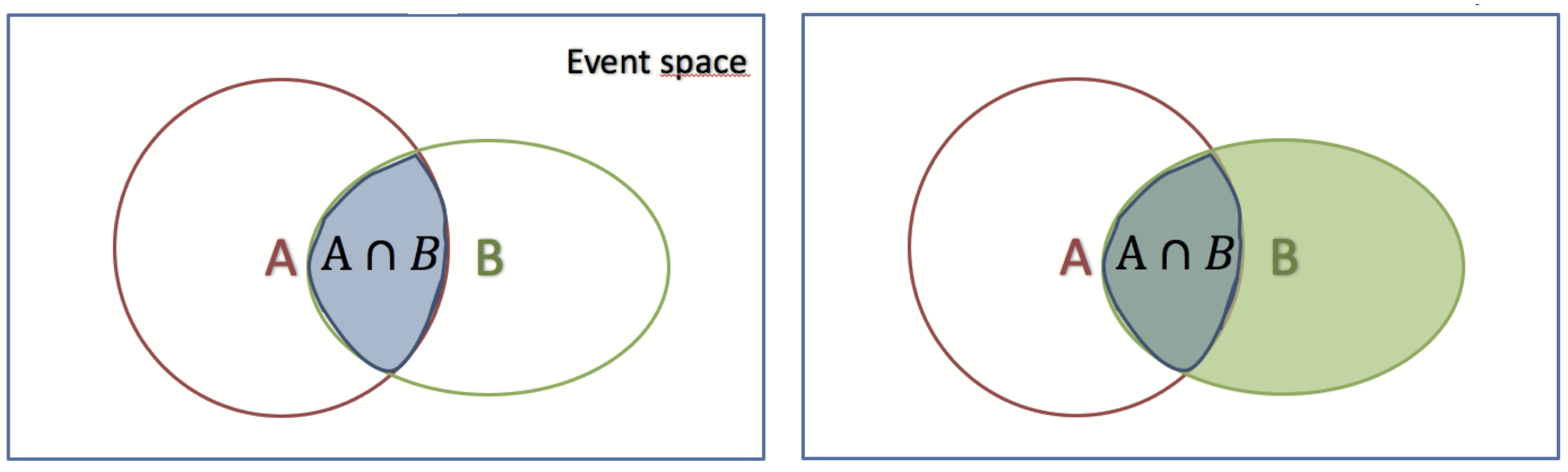
On the other hand a conditional probability is a measure of the probability of an event given that (by assumption, presumption, assertion or evidence) another event has occurred. If the event of interest is and the event is known (or assumed) to have occurred, “the conditional probability of given “, or “the probability of under the condition “, which is usually denoted as . A schematically illustration is given above right. The motivation for a conditional probability is that is sometimes useful to quantify the influence of a certain quantity onto another. Let’s look at examples from the everyday life: We want to know if smoking causes cancer . A logical implication would be , in words: smoking causes cancer ! But it is not that simple – finding even a single person which is a smoker and has not cancer falsifies our thesis. Nevertheless, while there exist smokers that have not cancer, there is a statistical relation between these two events: The probability to get cancer is higher if you smoke – this probability is the conditional probability . Generally speaking, given two events and , the conditional probability of given is defined as the quotient of the probability of the joint of events and , and the probability of : . This is called the Kolmogorov definition of the conditional probability. Note that in general , The relationship between and is given by Bayes‘ theorem: .
Self-Information & Entropy
In information theory, self-information or surprisal is a logarithmic quantity accounting for the amount of information, (or the entropy contribution) of a single message first defined by Claude E. Shannon the “father of information theory“. Or more practically: it is the minimum number of bits required to represent a message 1. The self-information is defined as . A plot of the self-information vs. probability is given below left. Here we have a nice example: The message “Mississippi” consist of characters with sample space {i,M,p,s} and the following corresponding probabilities of occurrence: and , which yields bit. Hence, we would need 21 bits for an optimal encoding of the message “Mississippi“.
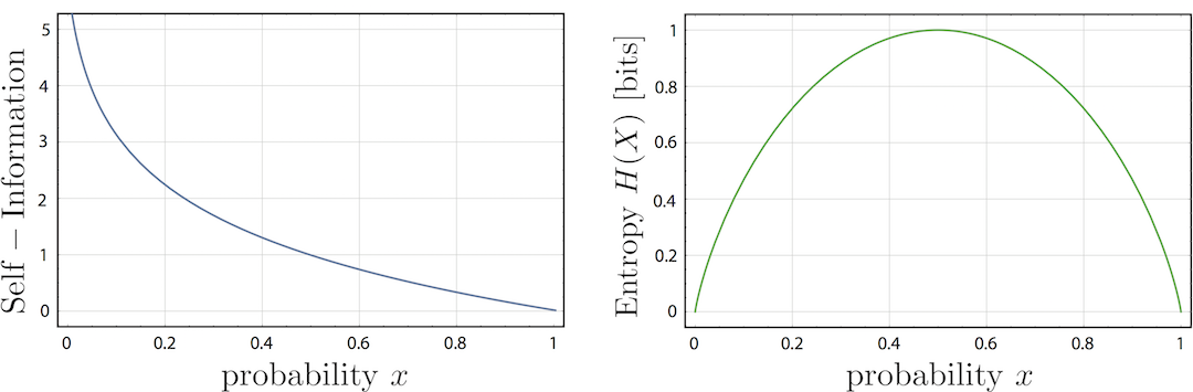
Closely related to self-information is the so-called Shannon entropy, which is the average (expected value) of the self-information, denoted as . For example if you do a fair coin toss – , we get bit – we gain the maximum possible amount of information (see plot above right for ). However, if the coin is biased – and the information received will be smaller than 1. If we already know the result of the coin toss prior for certain we will gain no information, . Finally a short Von Neumann-Shannon anecdote:
“My greatest concern was what to call it. I thought of calling it ‘information’, but the word was overly used, so I decided to call it ‘uncertainty’. When I discussed it with John von Neumann, he had a better idea. Von Neumann told me, ‘You should call it entropy, for two reasons: In the first place your uncertainty function has been used in statistical mechanics under that name, so it already has a name. In the second place, and more important, nobody knows what entropy really is, so in a debate you will always have the advantage. 2”
1. C. E. Shannon, Bell Labs Technical Journal, 27, 379–423 & 623–656 (1948). ↩