Is Heisenberg’s error-disturbance uncertainty relation violated? Experimental study of competing theoretical approaches

Theoretical Framework

Since our experiment verifying the theoretical findings of Masanao Ozawa, namely a violating and thus a necessary reformulation of Heisenberg‘s original error-disturbance uncertainty relation ¹, this particular field has experienced increased attention. However, soon after publication ², and reproduction of our results in photonics experiments ³, an alternative theory was presented by Paul Busch, and Pekka Lahti, and Reinhard F. Werner (BLW) ⁴ which in contrast stated the validity of Heisenberg’s relation and thus gave rise to heated debates. We carried out the first experimental comparison of these two competing approaches leading to a surprising result: Despite the strong controversy, in case of projectively measured qubit observables both approaches ⁵ even lead to equal outcomes ⁶.

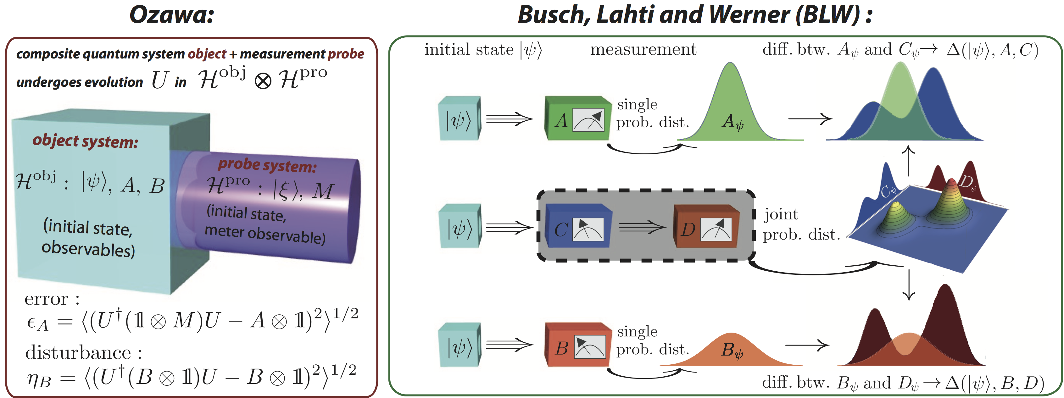
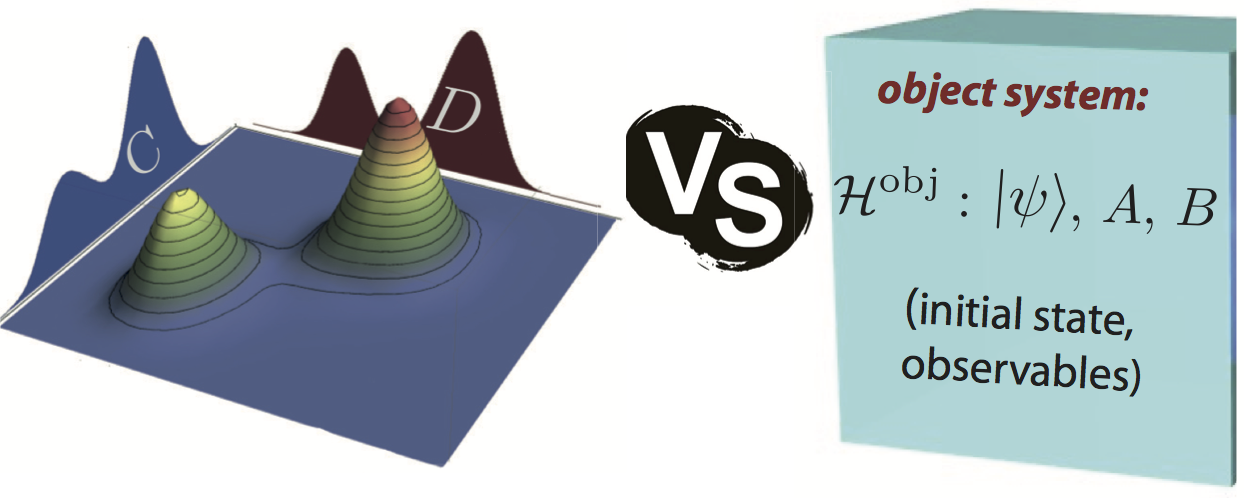
First let us start with a short comparison of the two approaches by M. Ozawa and Busch, Lahti and Werner (BLW): Ozawa’s approach, which is schematically illustrated above on the left hand side, makes use of a so-called indirect measurement model and is operator-based. Here, the measurement process is described by the interaction of a quantum object with a probe or measurement device. The object system’s Hilbert space is denotes as with observables and and initial state . The probe system’s Hilbert space then is with a meter observable and initial probe state . A unitary operator acton on accounts for the evolution of the composite object-probe system from its initially uncorrelated product state to the state after the measurement. Then, the measurement error is defined as root mean square deviation between observable before and meter observable after the measurement interaction . The disturbance induced on an observable by the measurement is given by the root mean square difference between that observable before and after the measurement interaction expressed as . Note that Ozawa’s error and disturbance are per se state-dependent quantities, as seen from the definitions above. However, in the case of qubit observables error and disturbance become state-independent.

In BLW’s approach, schematically illustrated above on the right hand side, error and disturbance are evaluated from the difference between output probability distributions. First accurate single measurements (reference or control measurements) of the target observables and in the input state are performed from which the probability distributions and are obtained. In a second step using a successive measurement scheme, the observable is first approximated by another observable denoted as , whose measurement induces a change of the input state and thus modifies the subsequent -measurement to be effectively a measurement of an observable on . Hence, the marginal distributions and of the joint probability distribution obtained from the successive measurement are compared with the output statistics of the single measurements. The difference between and defines the state dependent error and the difference between and is the state dependent disturbance both quantified by the Wasserstein-2-distance as and . Next BLW derive state in-dependent quantities from their state dependent expressions, which is in the qubit case achieved by worst case error/disturbance estimates.

Neutron Optical Experiment

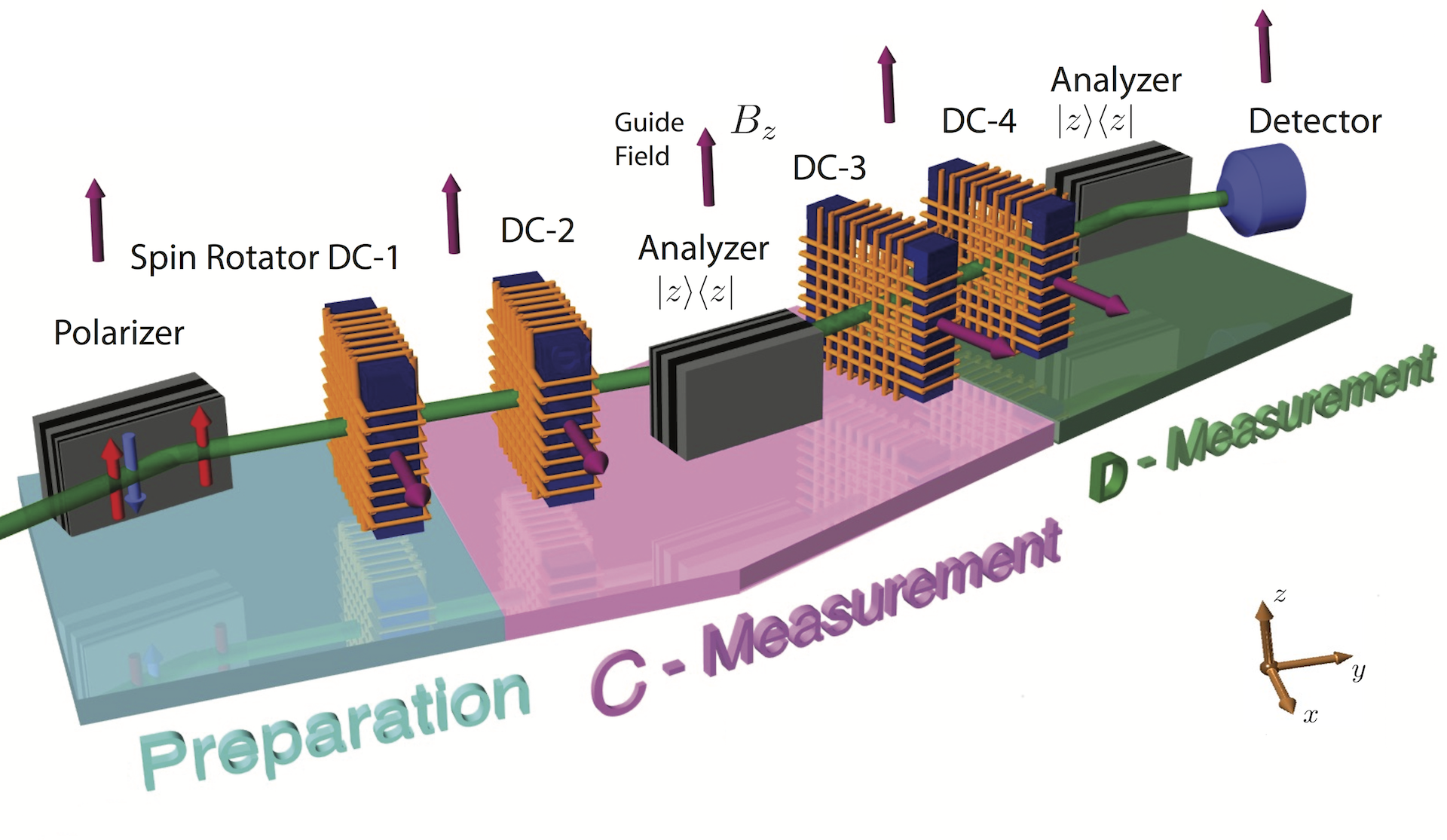
Below you can see our experimental setup for the successive measurement of two neutron spin observables  and  , and initial spin state  , with associated Bloch vector , where  denotes the vector of the Pauli spin matrices. Using supermirrors (as polarizer and analyzers) and exploiting Larmor precession, induced by the magnetic fields of guide field and spin turner coils DC-1 to DC-4, any required manipulation of the neutron spin can be performed. In our successive measurement, is approximated by another sharp but misaligned observable , with misaligmend (or detuning) parameter  as . Consequently the subsequent measurement is disturbed, which manifests by a transformation of the projectors into measurement operators as . The theoretically expected curves for Ozawa’s definitions simplify in qubit case to the state-independent expressions for error and disturbance . On the other hand BLW’s expressions for yet state dependent error and disturbance are expressed as and , respectively.

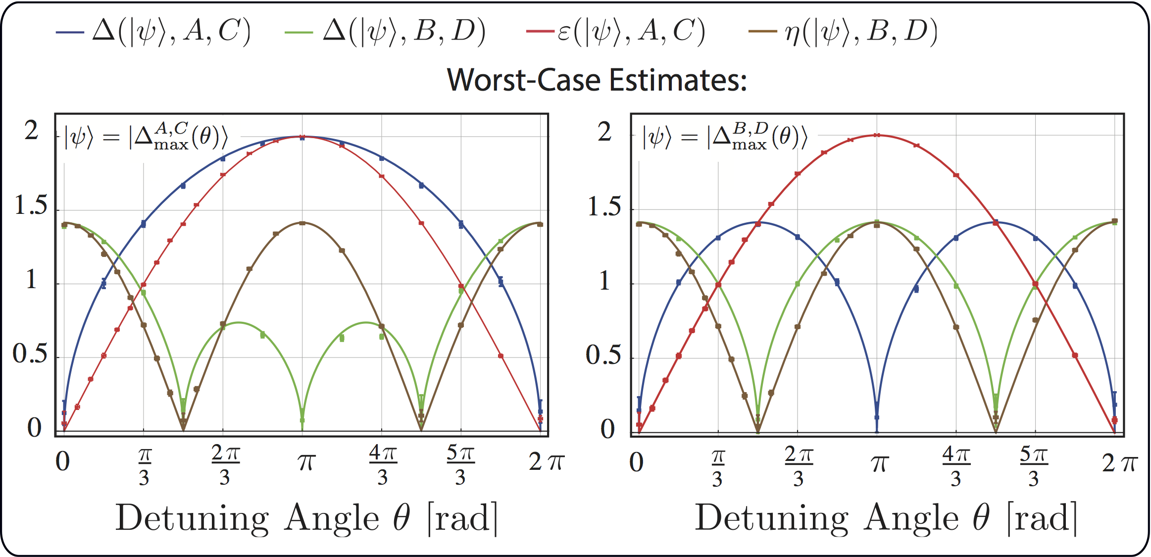
In the plots below our experimental results for , , , and are shown for different input states , suitable for illustrating the differences between both approaches and those necessary to construct BLW’s figures of merit are applied to successive measurement apparatus. In the very left plot the controversy concerning the state dependent disturbance becomes apparent. For , the approximator variable doesn’t modify the input states . BLW denote this configuration of the measurement apparatus as disturbance-free and vanishes. More precisely the initial states are so-called zero-noise, zero-disturbance (ZNZD) states, for which the first observable can be measured without noise and the second will not be disturbed, being a central part of the operational requirement (OR). Ozawa’s disturbance measure however requires more conditions to become zero. Another point of the debate between BLW and Ozawa becomes visible in the very right plot where the input state is chosen. Since its Bloch vector is perpendicular to the measurement axes , and all output probability distributions are equal. BLW argue that it is then natural to demand from a state dependent error/disturbance measure to vanish as is the case for and . Contrary, in Ozawa’s approach, equal probability distributions of target and approximator observable do not suffice to consider a measurement correct. Hence, neither nor vanish, but recognize the difference in the measurement operators even in a state where the probability distributions coincide, due to the tomographic measurement method (see here for details of the tomographic two-state-method), requiring a splitting up of the input state into auxiliary states.

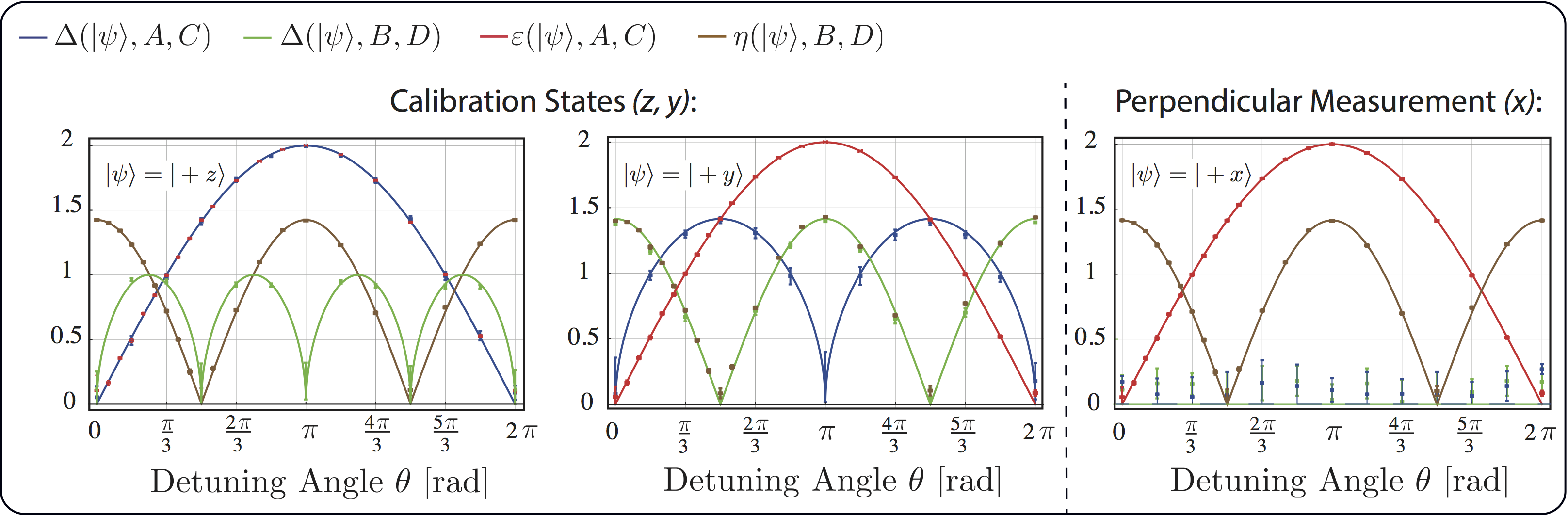
To get BLW’s state independent figures of merit special input states are required: The worst case error estimate is obtained from an input state with Bloch vector  maximizing , which is plotted below on the left side. The maximum   is achieved for an input state with Bloch vector and depicted below on the right side. Ozawa’s quantities of course remain unaffected by the choice of the input state. Thus we get and , where BLW’s and Ozawa’s and display the same extremal points and monotonic behavior. However, finding such global maxima for a measurement apparatuses requires in principle testing of all input states. We therefore favor the so-called calibration method, where the supremum is solely taken over input states for which the target observables have known and sharp values, which in our case for quits, these states are just the eigenstates of and of . BLW’s calibration error and disturbance thus coincide with Ozawa’s and , which can be seen in the above plot, left and middle panel for error () and disturbance (), respectively.

Final Results

To characterize the apparatus with respect to its overall error/disturbance performance, we thus have three different quantities: i) worst case estimates, ii) calibration errors/disturbances and iii) Ozawa’s quantities. For each configuration of the apparatus, the related pairs, denoted as i) ii) and iii) are compared in an error-disturbance plot below, together with the respective bounds and tested error-disturbance uncertainty relations.

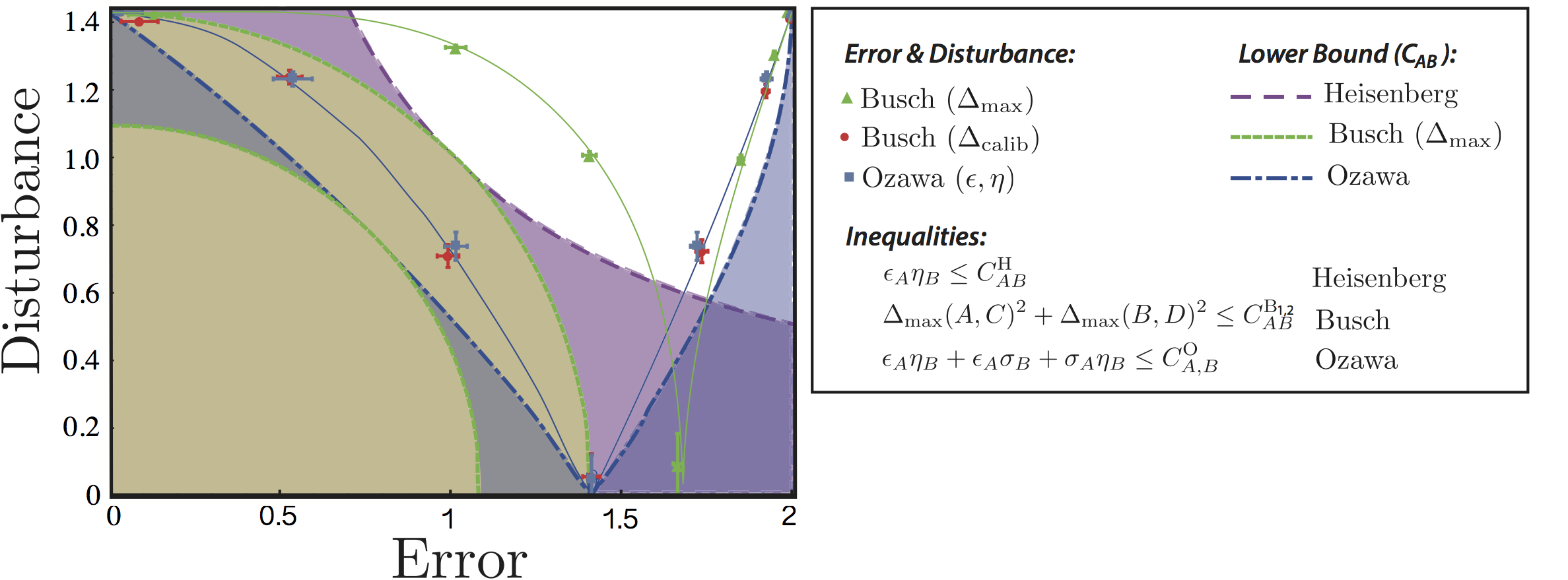 Error-disturbance points with either vanishing error or disturbance thus violate Heisenberg’s relation  with , which is the case for all three quantities.  Ozawa’s quantities and fulfill  Heisenberg’s relation only under limited conditions but always obey Ozawa’s reformulation , with  . Finally, for the worst case estimates and , BLW give a generally valid relation for qubit observables in terms of , where  quantifies the incompatibility of two qubit observables and is generally given by , and if the observable is sharp (), as in our case, ⁵.

1. M. Ozawa, Phys. Rev. A 67, 042105 (2003). ↩

2. J. Erhart, S. Sponar, G. Sulyok, G.Badurek, M. Ozawa, and Y. Hasegawa, Nature Physics 8, 185-189 (2012). ↩

3.  L. A. Rozema, A. Darabi, D. H. Mahler, A. Hayat, Y. Soudagar, and A. M. Steinberg, Physical Review Letters 109, 100404 (2012). ↩

4. P. Busch, P. Lahti, and R. F. Werner, Physical Review Letters 116 160405 (2013). ↩

5. P. Busch, P. Lahti, and R. F. Werner, Physical Review A 89 012129 (2014). ↩

6. Stephan Sponar and Georg Sulyok, Physical Review A 96 022137 (2017). ↩