Theoretical Framework

The issue of measurement is of fundamental significance in quantum mechanics which is applicable for the rather provocative title “How the Result of a Measurement of a Component of a Spin- Particle Can Turn Out to be 100″,¹  of a paper published by Yakir Aharonov, David Z. Albert and Lev Vaidman (AAV) in early 1988. In this paper AAV propose what they call a “new kind of quantum variable” which they gave the unique name weak value.

Contents:

Aharonov’s concept of Weak Measurements
””””Aharonov’s original experimental Proposal
Weak Values of two-level Quantum Systems
””””The quantum Cheshire Cat
””””The quantum Pigeonhole Effect – Violation of the classical Pigeonhole Principle
Weak Values obtained at arbitrary measurement strength
”””” Direct Measurement of the Quantum Wavefunction
”””” Generalized Eigenvalues

 Aharonov’s concept of Weak Measurements

Suppose an object system S, on which a Hermitian operator  shall be measured and a probe  system P (often refereed to as ancilla and sometimes measurement  device). An important point is that  both are considered being quantum systems, as illustrated below left. The weak measurement procedure involving three steps: (i) preparation of an initial quantum state   of the object system S, this is called pre-selection. (ii) a weak coupling of this system with a probe system P, with initial pointer state , via a coupling Hamiltonian . The initial state of the probe system P is supposed to be of Gaussian type (with initial spread  ), having a q- and a p-representation given by and , respectively. The observables is the canonical variable of the probe system, with conjugate momentum  and   is a function with compact support near the time of the measurement – normalized such that its time integral is unity. The interaction is supposed to be sufficiently weak, so that the system S is only minimally disturbed. Using the spectral decomposition of the initial state in eigenstates of  , given by   and   (eigenvalues ). The time evolution of the composite quantum system, consisting of both the object and the probe system is given by . Evaluating this expression yields an entanglement of probe and object system expressed as , which is a superposition a Gaussians (with width ) peaked at the eigenvalues .

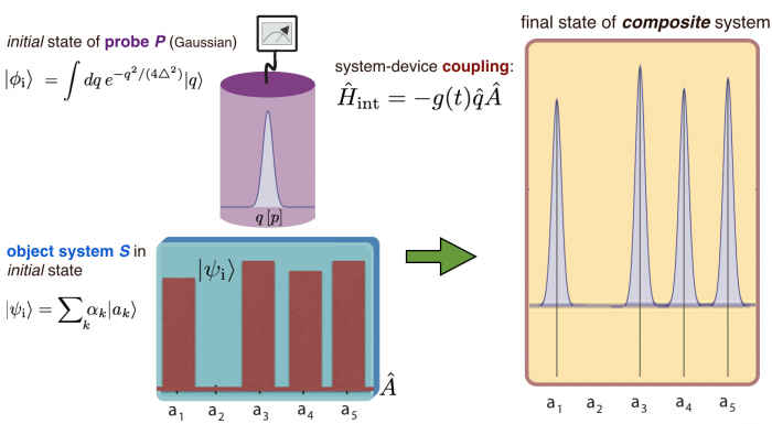
The probability distribution of the pointer states is given by . For this expression describes a usual strong measurement having the following three properties: i) the only possible measurement results are eigenvalues , ii) the probability of the outcome  is given by the squared amplitude , iii) if the measurement yields system left in the eigenstate .

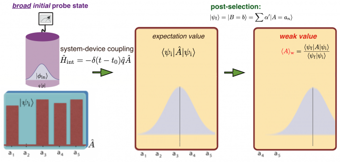
But what happens when the initial state of the probe system is broad ? In that case, instead of many peaks, we end up with a single peak , centered at the usual expectation value of   given by  . If a strong measurement of an observable  is performed in addition, the system in put in an definite final state , which is called post-selection. In the q-representation we get the following for the finial probe state:  , which is in p-representation. At this point AAV introduce an approximation for this sum of Gaussians that consist only of a single Gaussian centered at , where is called the weak value. The important condition is that the width of the initial probe state is broad compared to the mean difference of the eigenstates of , denoted as . Using this approximation the final probe states is calculated as

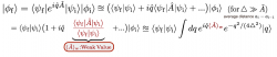
or .

At this point we want to take a look at a very simple example of the weak measurement, where a spin component of a spin- particle is weakly measured:

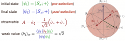
In a next step we calculate the output probability distribution of the final probe state for different values of the spread of the initial probe state. The animation below illustrates, that the AAV-approximation breaks down only for rather small values of the initial spread  ,i.e., .

 Aharonov’s original experimental Proposal

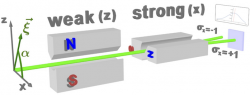
The original experiment proposed by Yakir Aharonov, David Z. Albert and Lev Vaidman (AAV) involves a beam of massive spin- particles. The observed quantum system is represented by the spin of a particle, while the probe system is formed by the particle’s spatial wave function. A schematic illustration of the measurement apparatus from the AAV gedanken experiments is given below A beam of particles, initially polarized in  -direction, where   is chosen to lie in the -plane with an angle in respect to the -axis.  The prepared (or initial) beam,  pre-selected with spin pointing in direction , passes through a weak magnetic field gradient, with the field pointing pointing in -direction. Here “weakly” means that the beams are still overlapping, hence one cannot get complete information of the spin direction (in  a strong measurement they would be clearly separated). The weak interaction causes a coupling of the spin with the two slightly shifted partial spatial wave functions correlated to the two values of . Next the beam passes another Stern-Gerlach apparatus, splitting it into two spatially separated sub-beams corresponding to . The weak value of   is determined from the post-selected  spin component, via the deflection of the spot on the screen in -direction. The -distribution of the spatial wave function is detected via counts observed on the distant screen and directly reflects the distribution of ‘s (momentum distribution) in the final beam.

 Weak Values of two-level Quantum Systems

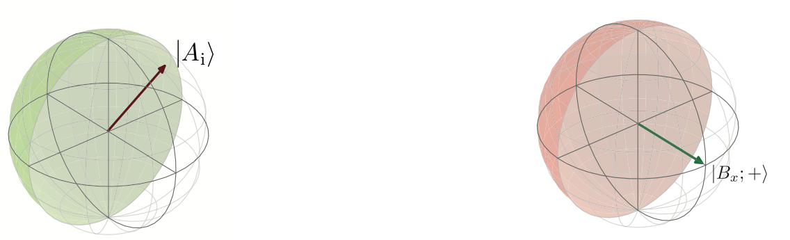
Assuming we have two two-level quantum systems and , referred to as system and . Each of the two quantum system is described by a two dimensional Hilbert space, which commute with each other. States aligned along the -direction are denoted as and for system and , respectively. the initial state of our composite system, consisting of system that shall be weakly measured and system , accounting for our probe or measurement system is prepared to be given by . Now the initial state of the probe system is chosen to be aligned along direction, yielding , a completely separable state – no coupling at all – as illustrated below. As a next step a coupling is created by the interaction Hamiltonian the condition for a weak measurement is fulfilled by making sufficiently small ².

The interaction Hamiltonian causes an evolution of the system state vector from an initial state to the evolved state denoted as , where we used the first two terms of the exponential function’s Taylor series (or expansion)  – valid only for small and , the flip bit operation.

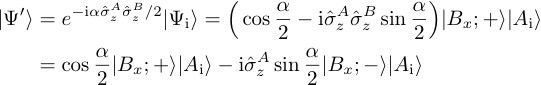
Next we post-select onto a final state , generally expressed as , with and denoting polar and azimuth angle on the Bloch sphere of . Then the final state of the composite system reads

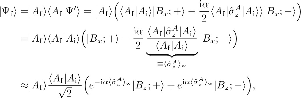
after re-exponentialization. Now taking into account that the weak value is in general a complex quantity, meaning , we see that the weak value of gets “encoded” in the system : The real part of the Pauli operator’s weak value acts as an additional phase shift, i.e. a longitudinal move, of the state vector, whereas the imaginary part causes a change in the weight, i.e. a latitudinal shift as illustrated below:

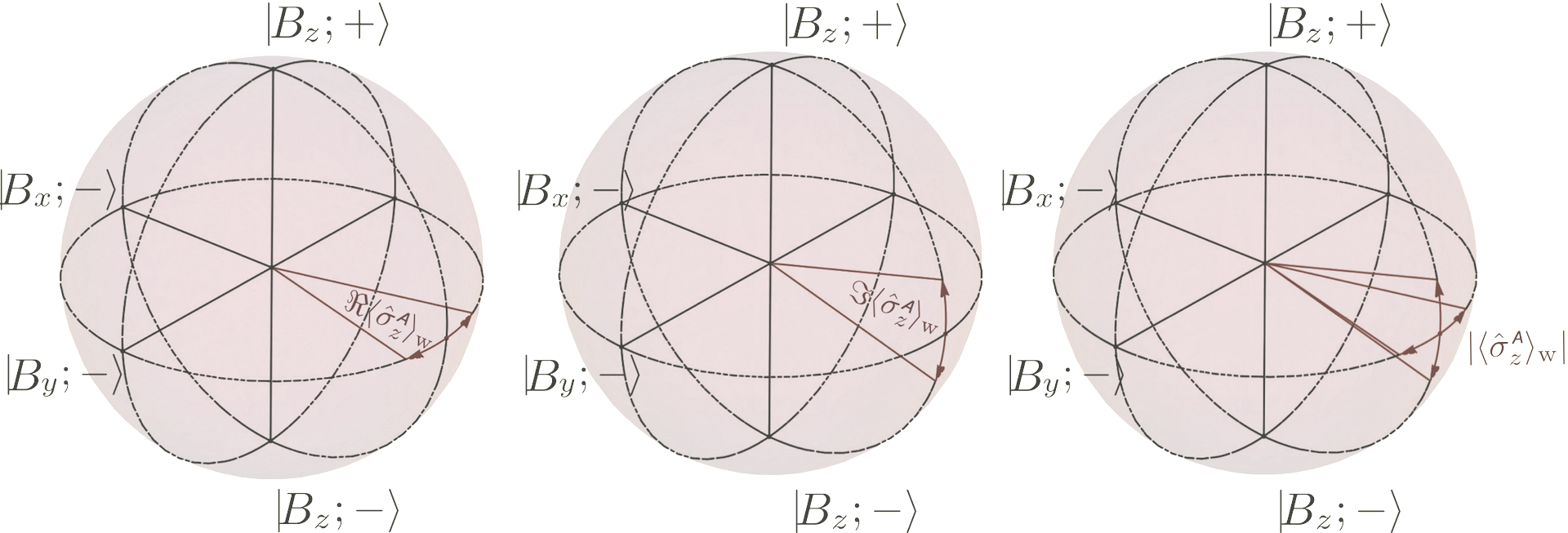
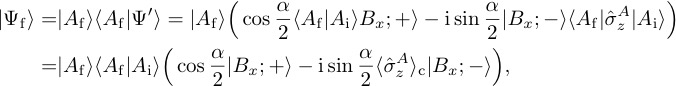
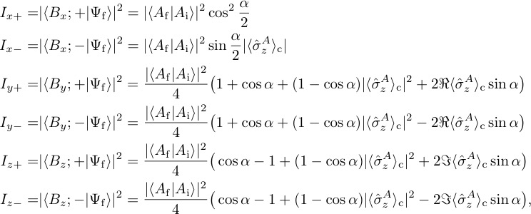
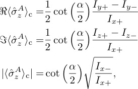
The real and imaginary part as well as the modulus of the weak value of the Pauli operator, associated with system and denoted as , can now be extracted by evaluating the expectation values of the three Pauli operators of , namely and , which can be expressed using the six intensities and given by:

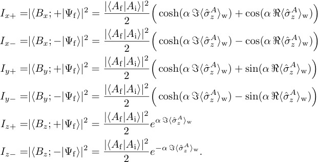
Combining the results for the intensities yields

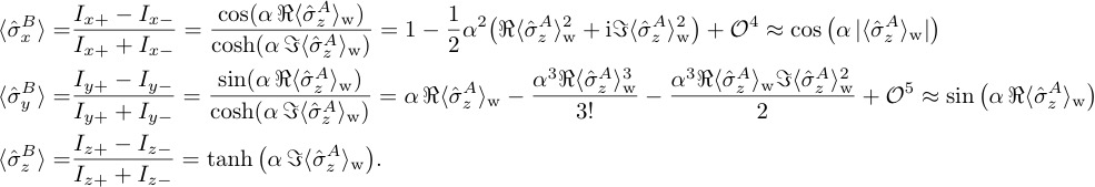
Finally the relations

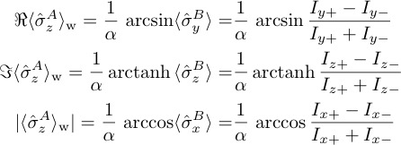
hold up to the first order in . Details of our neutron interferometric experiments, where quantum systems  and  are represented by the neutron’s spin and path degree of freedom can be found here.

 The quantum Cheshire Cat

Everybody knows the famous Cheshire cat from Alice in Wonderland (complete title Alice’s Adventures in Wonderland), either by reading Lewis Carroll’s (whose actual name was Charles Lutwidge Dodgson) novel or from one of the various motion pictures or the Walt Disney‘s animated adventure-film. The peculiarity of the Cheshire cat is that from time to time its body disappears, while its iconic grin remains visible. In the quantum Cheshire cat, a paradox proposed by Yakir Aharonov ³ 2013, the cat is substituted by the particle itself and the cat’s grin is replaced by the spin component. It is now possible to create a pre and postselected quantum ensemble that behaves in average as if the particle and its spin component are spatially separated – a disentanglement of a particle from one of its properties: While the particle (the cat) take the upper beam path their spin  (the grin) travel along the lower one.  An artistic depiction of this behavior is shown below.

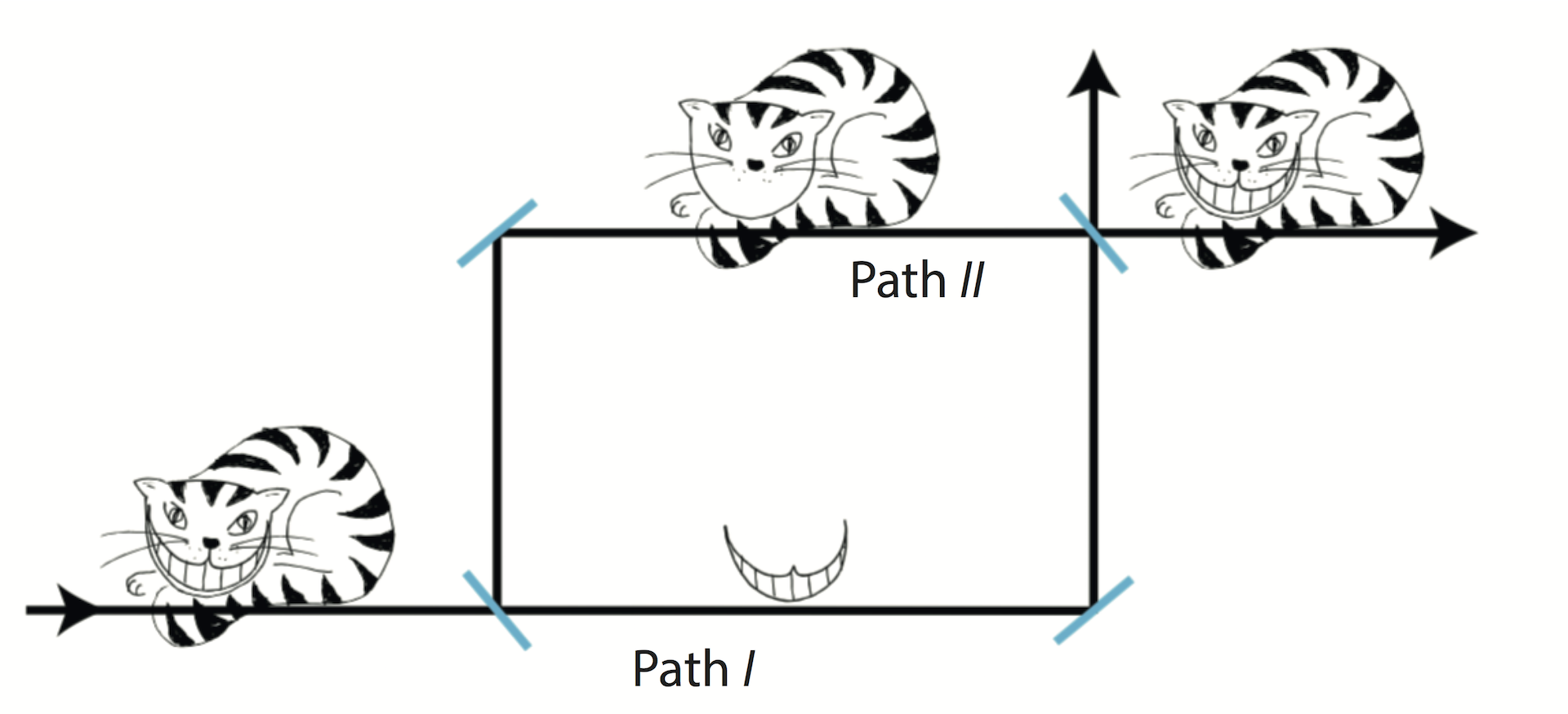
In order to create a quantum Cheshire cat the initial state has to be pre-selected in a state is given by a superposition of the two path eigenstates (path & path ) with orthogonal spin states, i.e., a Bell state expressed as . The system’s post-selected state is given by the separable state . Asking about the location of the particle between pre- and pos-selection we have to calculate the weak values of the path projection operators expressed as . Asking for the location of the particle we have to calculate the weak value of the path projection operators, yielding   and . Hence, the system’s state vector will behave as if there were no particle traveling along path () but only along path (). Furthermore, sine the operators   are dichotomic operators (that is an operator having only two eigenvalues), this result will also hold in the strong limit, because it can be shown that if the weak value of a dichotomic operator equals one of its eigenvalues, then the outcome of a strong measurement of the operator is that same eigenvalue with probability one ⁴.

To get the  path of the grind, the particle’s property, we have to calculate the weak values of the operator product  , i.e., the spin’s -components conditioned on the path, which gives  and . This result tells us that in the weak regime any coupling to the particle’s spin’s -component is only effected on path () while there is no effect on path (). At the same time we found that a coupling to the spatial part of the wave function is only effective along path . We can create a quantum ensemble that behaves in average as if it were separated from one of its properties: a quantum Cheshire cat emerges. See here for our neutron interferometric realization of the quantum Cheshire cat experiment.

 The quantum Pigeonhole Effect – Violation of the classical Pigeonhole Principle

The pigeonhole principle, first stated by Dirichlet in 1834 and therefore also reffered to as Dirichlet’s box principle or Dirichlet‘s drawer principle (“Schubfachprinzip“), states the following: “If you put three pigeons in two pigeonholes, at least two of the pigeons end up in the same hole.”Or in a slightly more mathematical style: “if items are put into m containers, with , then at least one container must contain more than one item“. It is an obvious and fundamental principle of nature as it captures the very essence of counting. It can for instance be utilized to demonstrate there must be at least two people in New York City with the same number of hairs on their heads. Since a typical human head has an average of around 150 000 hairs, it is reasonable to assume (as an upper bound) that no one has more than 1 000 000 hairs on their head ( = 1 million holes). There are more than 1 000 000 people in New York ( is bigger than 1 million items). Assigning a pigeonhole to each number of hairs on a person’s head, and assign people to pigeonholes according to the number of hairs on their head, there must be at least two people assigned to the same pigeonhole by the 1 000 001st assignment (because they have the same number of hairs on their heads) (or, ). In the quantum version of the pigeonhole principle, a paradox proposed by Yakir Aharonov ⁵ in 2016, the pigeons are replaced by particles and the two boxes by the path of an interferometer, which is schematically illustrated below.

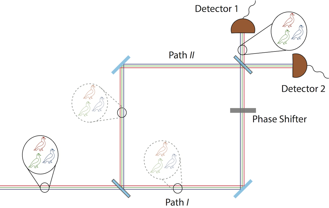
Consider three particles and two boxes, associated with Path and in an interferometer, each particle prepared in a superposition of the two pathes, denoted as . The overall initial state of the three particles is therefore given by . At this point it is obvious that in this state any two particles have nonzero probability to be found in the same box (path). However, to find instances, where no two particles are together, we subject each particle to a second measurement, wherer we measure whether each particle is in the state or . We are interested in the state, yielding a finial overall state expressed as . Note that neither the initial state nor the finally selected state contains any correlations between the particles, we have three non-interacting, non-entangled, uncorrelated particles. Let us now check whether two of the particles are in the same box (since the state is symmetric, we could focus on particles 1 and 2 any result obtained for this pair applies to every other pair). Particles 1 and 2 being in the same box means the state being in the subspace spanned by and (being in different boxes corresponds to the sub-spaces spanned by and ). The projectors corresponding to these subspaces are and , with , , and . On the initial state alone, the probabilities to find particles 1 and 2 in the same box and in different boxes are both , on the other hand, given the results of the final measurements, we always find particles 1 and 2 in different boxes – a violation of the classical    pigeonhole principle which we call the quantum pigeonhole effect. Here is the explanation: suppose that at the intermediate time we find the particles 1 and 2 in the same box, which means , which is orthogonal to the postselected finial state and therefore . Thus in this case the final measurements cannot find the particles in the state and therefore, the only cases in which the final measurement can find the particles in the state are those in which the intermediate measurement found that particles 1 and 2 are in different boxes (paths). See here for our neutron optical experimental demonstration of the quantum pigeonhole effect.

 Weak Values obtained at arbitrary measurement strength

As before the system’s preselected sate vector given by . However, instead of performing a series expansion around the exact formula is used. The action of the evolution operator then gives

The postselection on the the final state then leads to

where denotes the contextual value of the Pauli operator , valid for all values of , i.e., for arbitrary measurement strengths. Again calculating the the six intensities  and yields

and combining them finally gives

being the real and imaginary part and the modulus of the weak value of the Pauli operator , holding for all values of . See here for our neutron optical experiment studying weak values obtained at arbitrary measurement strength.

 Direct Measurement of the Quantum Wavefunction

In 2011 a novel direct tomographical method was presented ⁶ which made it possible to determine the quantum state without the need for post-processing, as it it the case for quantum state tomography (see here for details on tomography). The basic principle of the direct measurement of a quantum state is the following: general representation of a state vector is given by , with eigenstates and probability amplitudes . If we now calculate the weak value of a projection operator onto an eigenstate we have the usual expression . Pluggin in the definition of th eprojection operator from above we get , where the deninition of the probability amplitudes occours and after rearranging the terms we get an expression of the probability amplitudes in terms of weak values . For the complete state vector we nowhave the expression . See here for our direct measurement of the neutron’s path state in the interferometer.

 Generalized Eigenvalues

In the original framework of weak measurements, as developed by Yakir Aharonov, David Z. Albert and Lev Vaidman (AAV) ¹, the formula for the weak value only applies to pure initial and final states, and even more important here, with weak measurement strength. Naturally the following question arises: “Is the weak value expression still operationally meaningful for impure boundary conditions and arbitrary strength measurements ?” This question was addressed in by Andrew N. Jordan and Justin Dressel by introducing the concept of  contextual values of an observable, as a generalization of its eigenvalues that take into account the details of the specific measurement procedure ⁷. However, the term has caused confusion with the unrelated concept of contextuality as it applies to hidden variable models of the quantum theory. We therefore referre to these values as generalized eigenvalues. Even for non-projective measurements one may still assign meaningful values to imperfectly correlated detector outcomes—that is, averaging carefully chosen values can recover the correct expectation value as an ensemble average, but the needed values are generally not eigenvalues. This equivalence under the averaging process can be expressed more formally in terms of an operator identity, , where are the eigenvalues of with eigenstates and are contextual values for with respect to a particular positive operator-valued measure (POVM) , satisfying  (see here for an introduction towards POVMs).

It can be shown how conditioned averages of generalized measurements converge to the weak value as a stable limit point when the measurements become sufficiently weak ⁷. For purity-preserving measurements such that the POVM elements factor into single Kraus operators , a general conditioned average of generalized measurements in between an initial mixed state and a final generalized measurement POVM will have the form ,where the perturbation away from a generalized weak value expression is determined by Lindblad decoherence with . In the case of a weak measurement, , the commutators in the Lindblad disturbance approximately vanish, leaving the weak value expression as the conditioned average. Evidently from this analysis, it is clear that any situation in which the Lindblad disturbance can be made irrelevant in the numerator will be able to recover a generalized weak value as an operational average, up to renormalization. It thus becomes interesting to consider special cases where stronger measurement strengths with less statistical uncertainty can recover the weak value expression without any approximations. See here for our experimental study of generalized eigenvalues in an neutron interferometric experiment.

1. Yakir Aharonov, David Z. Albert, and Lev Vaidman, Phys. Rev. Lett. 60, 1351–1354 (1988). ↩

2. T. Denkmayr, PhD Thesis: Experimental investigation of weak values in massive quantum systems (2016). ↩

3. Y. Aharonov, S. Popescu, D. Rohrlich, and P. Skrzypczyk, Quantum Cheshire Cats, New Journal of Physics 15, 113015 (2013). ↩

4. Y. Aharonov and L. Vaidman, Journal of Physics A 24, 2315 (1991). ↩

5. Y. Aharonov, F. Colombo, S. Popescuc, I Sabadini, D. C. Struppa, and J. Tollaksen, Proc. Natl. Acad. Sci. USA 113, 532 (2016). ↩

6. J. S. Lundeen, B. Sutherland, A. Patel, C. Stewart, and C. Bamber, Nature (London) 474, 188 (2011). ↩

7. J. Dressel, S. Agarwal, and A. N. Jordan, Phys. Rev. Lett. 104, 240401 (2010). ↩