Contextually and The Kochen-Specker Argument
October 5, 2016 1:05 pmThe Kochen–Specker, also known as the Bell–Kochen–Specker theorem, represents an important and subtle, topic in the foundations of quantum mechanics. The theorem demonstrates the impossibility of a certain type of interpretation of quantum mechanics in terms of hidden variables, trying to explain the apparent randomness of quantum mechanics as a deterministic model featuring so-called hidden states. Beside the common Copenhagen interpretation of quantum mechanics there hidden – variable theories have been introduced, as a possible consequence of the EPR-Paradox, to maintain a realsitc world-view. Most of them can be eliminated by so called “no-go theorems” for hidden variables – the most famous of them is Bell’s theorem. The Kochen-Specker theorem complements Bell’s Inequality and excludes contextuality (in addition to locality) from hidden-variable theories. The Copenhagen interpretation is named after the Danish capital, where Niels Bohr and Werner Heisenberg were exchanging their thoughts about the probabilistic interpretation of the wave function. Although there is no clear statement about this interpretation of quantum mechanics at the heart of this idea is the idea that the wavefunction has no reality. Consequently nature is only probabilistic and only a measurement forces it to choose a state. So befor the measurement there is no reality, the process of measurement causes a collapse of the wave function.
Contents:
Proof of original Kochen-Specker (KS) Theorem in three Dimensions with 117 Vectors
”””” Peres’ proof in three dimensions with 33 vectors
”””” Peres’ proof in four dimensions using 24 vectors and Mermin’s magic square
ψ-ontic & ψ-epistemic Models – Reformulation of Contextuality
”””” An operationlal definition of contextuality for preparations, transformations, and unsharp measurements
Proof of original Kochen-Specker (KS) Theorem in 3 Dimensions with 117 Vectors
The original KS (oKS) proof, as given in paper from Simon B. Kochen and Ernst Specker published in 1967 1, operates on a three-dimensional complex Hilbert space . It requires the following two assumptions: (1) sets of triples of rays which are orthogonal in ; (2) a constraint to the effect that of every orthogonal triple one ray gets assigned the number 1, the two others 0.
Let be projecting on the rays spanned by the eigenvectors of an arbitrary operator defined on . Since are mutually compatible, we can apply the Sum Rule and Product Rule, yielding the following constraint on the assignment of values:
oKS1: where or , for .
Proof: Since the projection operators form an orthonormal basis applies and from the Sum Rule follows. According to the Product Rule and the fact that projection operators are idempotent gives as only possible values or . Finally, assuming an observable and applying again the Product Rule we get , which gives .
We introduce incompatible observables . which select different orthogonal triples in . Assumption OKS1 tells us that every one of these triples has three values, namely exactly {1, 0, 0}. Now the argument is the following: It is impossible for a specific finite set of orthogonal triples in to assign numbers {1, 0, 0} to every one of them.
It should be stressed that while is complex, it is enough here to consider a real three-dimensional Hilbert space . This is so because if the assignment of values according to oKS1 is impossible on , then it is impossible on as well. It is worth noting at this point there is no direct connection between the three-dimensional (real) Hilbert space and physical space . In particular, orthogonality in should not be confused with orthogonality in physical space , as the following example demonstrates: Considering an arbitrary direction in physical space and an operator representing the observable of a spin component in direction . The corresponding Hilbert space in turn is spanned by the eigenvectors of , namely , and , which are mutually orthogonal in the Hilbert space.
At this point KS surprisingly choose to illustrate this with an example that does in deed establish a direct connection with physical space: they consider an atom in a triplet state, which forms a single-particle spin-1 system. The operators describing the spin are given by the Pauli spin matrices for S=1:

These observables are non-commuting, while they have all the same eigenvalue spectrum their eigenvectors are different:

However, the squared components of the spin and , given by

are compatible, i.e., mutually commuting, they have a common set of eigenvectors (for different eigenvalues)

So the following three measurement outcomes are possible: or . So in whatever direction is measured the result of three squared spin Operators will yield once 0 and two times 1, which leads to the second constrain:
oKS2: where or , for .
Proof: Since and are the usual angular momentum operators satisfying and the eigenvalues of are . For we get , where denotes the identity operator. by applying Sum and Product Rule (as in oKS1) we end up with oKS2 from above.
Now we can define an observable of type and a specific choice of in turn selects three orthogonal rays in physical space, that is by fixing a coordinate system. Now numbers {1, 1, 0} have to assigned to due to the specific choice of O or — more precisely to and — which of course is the mirror-image of our previous problem of assigning numbers {1, 0, 0}. So in this example orthogonality in does correspond to orthogonality in physical space (the same holds also for ). Nevertheless this correspondence is not necessary to proof the argument ! The KS proof shows that it is impossible to assign to the spin-1 particle values for all these arbitrary choices, or in other words: a spin 1 particle cannot possess all the properties at once which it displays in different measurement arrangements.
A given point on the unit sphere uniquely picks out a unit vector from the origin to which in turn uniquely picks out a ray in physical space through the origin and denoted as . Another vector (ray) enclose an angle . Now suppose a vector orthogonal to , and also orthogonal to (see image below left side). Moreover, the direction of is such chosen that is the angle between and given by .

KS diagram and directions in real space
The corresponding KS diagram is depicted above on the right side. A KS diagram is realizable on a unit sphere, if there is a 1:1 mapping of points on the unit sphere (vectors in ) to vertices of the diagram such that the orthogonality relations in the diagram, i.e., vertices joined by a straight line represent mutually orthogonal points, are satisfied by the corresponding vectors. The following ten-point KS diagram is realizable if and only if the vectors and are separated by an angle with .

Ten-point KS graph T1
Proof: Suppose and which, together with form a complete set of orthonormal vectors. Then being orthogonal to can be expressed as , a normalized vector in the plane spanned by and with arbitrary real number . In the same manner being orthogonal to is given by . Next applying the orthogonality relations in the KS diagram from above yields and . Since is orthogonal to ) and we get , which results in . Similar we get . Since the inner product of two unit vectors just equals the cosine of the angle between them one can write and since we get finally get , which has a maximum value of 1/3 for . So the diagram is realizable for .

(left) Ten-point KS graph T1 with inconsistent coloring (right) with consistent colouring
Now we come to the coloring problem: colour the points white (for “0”) and black (for “1”). The constrains from above can be translated in the following problem of colouring the vertices: One has to colour the diagram white or black such that joined vertices cannot be both white and triangles have exactly one white vertex. At this point we assume that and have different colors, then the colouring constraints force us to colour the rest of the diagram as depicted above on the left side . However, this requires that and are orthogonal and both have are white, which is forbidden. Hence, two points closer than cannot have different colors (a possible correct coloring, which is consistent with the constraints is depicted above on the right side).
Next KS construct another quite complicated KS diagram in the following way by considering a realization of T1 for an angle . Then they choose three orthogonal points and spacing interlocking copies of T1 between them such that every instance of point of one copy of T1 is identified with the instance of of the next copy. Five interlocking copies of T1 are spaced between and , which trace out an angle of 5×18° = 90° which is exactly what is required so that and can be connected by a vector, which is schematically illustrated below. As seen from above for each of these 15 vectors, which are depicted on the unit sphere below, it is possible to find 8 orthogonal vectors.

The famous 117 vectors KS graph T2 with cannot be consistently coloured
However, although T2 is constructible it is not consistently colorable ! Since in one copy of T1 is identical to in the next copy, in the second copy must have the same colour as in the first, so all instances of must have the same colour. and are identified with points , so they must be either all white or all black — but since and form an orthogonal triple exactly one of them must be white !
Peres’ 33 vector proof
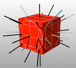
Kochen and Specker’s ingenious argument was to consider the squared spin in just a handful of directions. The simplest version of their result, discovered by Asher Peres and published in 2, drew two lines dividing each face in quarters, then drew the largest possible circle on each face, and inside of each of these circles drew the largest possible square. We only use directions from the particle at the centre of the cube to the intersections of these markings on the faces. So in total we get 9 intersections on each of the 6 faces and an additional point on the middle of each of the 12 edges, which creates 66 directions from the centre of the cube. But since the squared spin is the same in opposite directions, Peres really only had to take 33 directions into account. The 101 property as a coloring problem: Consider measuring the squared spin of a particle in the three perpendicular directions along the positive x, y, and z axes, as depicted below. Suppose it is 1 in the positive x-direction (shown as the black axis pointing out of the page), 0 in the positive y-direction (show as the white axis pointing to the right), and 1 in the positive z-direction (the black axis pointing upwards). Then, again by the 101 property, squared spin of the particle will be 0 in every direction perpendicular to the first white bar. If you assume that the squared spin of the particle has a definite value in all of these directions, you end up with a contradiction, which is illustrated below – the squared spin in one direction ends up being both 0 and 1 – black and white (indicated by the blue bar).
Geometric proof of KS theorem in three dimensions
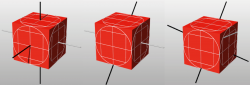
Let’s look at this step by step: first we have to satisfying the 101 property (left). For example, the squared spin will be 1 in the direction from the particle to the middle of the top-rear edge of the cube (middle). Third direction, through middle of the top-rear edge of the cube, is mutually perpendicular with to the bars through the top-left and bottom-right corners of the squares on the right-side face of the cube (right).
Then, by the 101 property, the squared spin will be 1 in any direction perpendicular to the top-left bar through the right-side face. For example, the bar through the middle-left side of the square on the front-side of the cube will be black (left). Then this black middle-left bar through the front-face of the cube is perpendicular to the previous black bar through the centre of the top face. These bars are mutually perpendicular to that through the middle-left of the right-side face, and this bar must therefore be white (middle). Then by the 101 property all bars perpendicular to this white bar must be black – including the top-left and bottom-left bars through the front face of the cube (right).
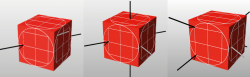
Then the bottom-left and top-right bars through the front face of the cube are mutually perpendicular to the bar through the middle of the top-left edge of the cube – this bar must be white (left). Similarly, the top-left and bottom-right bars are mutually perpendicular to the bar through the middle of the top-right edge of the cube. Therefore this bar must also be white (middle). The white bar through the middle of the top-left edge of the cube is perpendicular to the bar through the middle of the top-right edge, which implies that this bar must be black. But we have just seen, shown in the picture above, that this bar must be white. And we have reached a contradiction: this bar (shown in blue) must be both black and white (right).
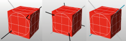
“If the answers were chosen ahead of time you could stick bar through each of these directions,” says Conway. “Thirty-three bars: a black bar if the predetermined answer was 1 and white if the answer was 0. But [Kochen and Specker showed that] it is impossible to label all these directions with 1’s and 0’s so that they all satisfy the 101 rule; you get to a point when you need both a black and white bar.”
The way Peres gave the proof in his paper is the following: “The 33 rays are those for which the squares of the direction cosines are one of the combinations and all permutations thereof.” 2 The rays are labeled , which can have values (which means -1), 2 (), (). So for example the ray connects the origin with the point and the squares of the direction cosines are and . Ray printed in italic are “old”, i.e., were found to be black in a line before. Opposite rays (denoting the same direction in space), such as for instance and are only counted once. The 33 vectors are given in the table below left and the proof is given on the right side (only rays needed for further work, namely 25, are listed in the original proof given in 2. The reason for that us the specific choice of the z-axis – the “unused” rays are marked with an asterik in the left table):

The 33 Peres rays and proof of KS theorem in three dimensions
The rays , and (market red) are black and mutually orthogonal. This is the KS contradiction. Note that if only one of the 33 rays is removed the contradiction disappears.
Peres’ 24 vector proof in four dimensions
Using the same notation as before 24 rays in labelled are , ,, , , and all permutations thereof. This set is invariant under interchanges of and and under reversal of the direction of the each axis. The table below proves the KS theorem for this case.

Proof of KS theorem in four dimensions
The rays , , and (marked red) are black and mutually orthogonal: again a contradiction. All 24 rays appear explicitly in the table – of a single one is deleted the contradiction can be avoided. A peculiarity of the 24 rays in is that the rays form six disjoint orthogonal tetrads. From the four projection operators corresponding to each tetrad one obtains . These three operators form a complete set of commuting operators. If one tries to assign numbers (+1 or -1) to each operator in such way that the product of this three operators is equal to the product of the operators in each tetrad a contradiction arises. The simplest way to see this an concrete example: consider pair of spin- particles. In the square

Peres magic square
each row and each column is a train of commuting operators, as discussed above 3. The KS contradiction arises due to the fact that the product of the three operators in each column or row is , except the that of the third column which is . It is obviously impossible to assign numbers (+1 or -1) to each of the nine operators reproducing this result.
ψ-ontic & ψ-epistemic Models – Reformulation of Contextuality
Let’s dive directly into it and start with the heated discussed qustion whether the quantum state must be ontic, which means a state of reality, rather than epistemic, being a state of knowledge. The word “ontology” derives from the Greek word for “being” and refers to the branch of metaphysics that concerns the character of things that exist. In the context of quantum mechanics this means that an ontic state refers to something that objectively exists in the world, independently of any observer (or agent). On the other hand, “epistemology” is the branch of philosophy that studies of the nature of knowledge (information or belief). An epistemic state is therefore a description of what an observer currently knows about a physical system it therefore exists in the mind of the observer rather than in the real world (our universe). So when a quantum state is assigned to a physical system, does this mean that there is some independently existing property of the individual system that is in one-to-one correspondence with , or is simply a mathematical tool for determining probabilities, existing only in our minds ?
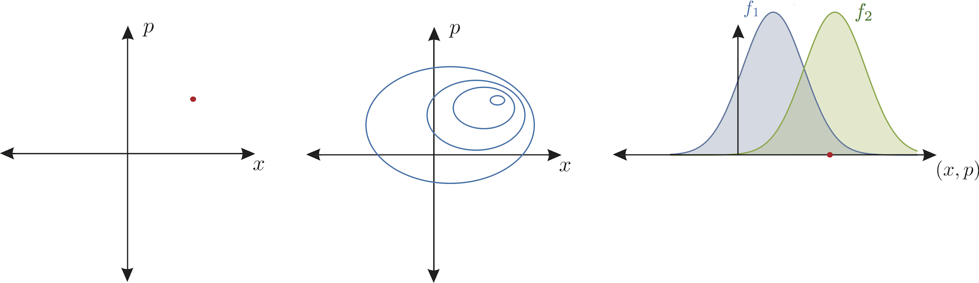
In classical mechanics, the distinction between ontic and epistemic states is quite simple: a single Newtonian particle in one dimension has a position and a momentum and these are objective properties of the particle that exist independently of our mind. the particle’s ontic state is a point in phase space, which is illustrateds below on the very left side. An epistemic state, on the other hand, is a probability density in phase space (contours indicate lines of equal probability), plotted in the middle for an epistemic state denoted as . Note that a single ontic state (red point) is deemed possible in more than one epistemic state, in our example for the two epistemic states and , which is plotted on the very right side below.
-epistemic interpretation
Before getting into the details of –epistemic explanations, it is important to distinguish two kinds of –epistemic interpretation: First we have the Neo-Copenhagen approch, who’s advocates (like in the original Copenhagen interpretation bearing the views of Niels Bohr, Werner Heisenberg and Wolfgang Pauli) deny the need for any deeper description of reality beyond quantum theory – typical -epistemic opinion. Modern neo-Copenhagen views include the Quantum Bayesianism (QBism: the wave function does not describe the world — it describes the observer who is updated by an agent) developed by Carlton M. Caves, Christopher Fuchs and Rüdiger Schack, as well as the views of David Mermin, Asher Peres, and Anton Zeilinger. The second type of –epistemic interpretation are those that are realist, in a sense that they postulate at least some underlying ontology. There is evidence that Albert Einstein‘s as well as Stuart Ballentine‘s view was of this type. More recently, Robert W. Spekkens has been a strong advocate of this point of view 4. Just a short side remark; realistic –epistemic interpretations are already strongly constrained by existing no-go theorems, just to mention Bell’s theorem and the Kochen–Specker theorem. In 4 Spekkens introduced a toy theory that qualitatively reproduces the physics of spin-1/2 particles, when prepared and measured in the , and bases, which is explained here in detail.
-ontic interpretation
There are a handful of fully worked out realist interpretations of quantum theory, most prominent candidates are many-worlds theory and de Broglie–Bohm theory, where in each of these interpretations the wavefunction is part of the notice state. According to Richard Feynman, single particle interference phenomena, such as the double slit experiment, contain the essential mystery of quantum theory – or in his own famous words: “We choose to examine a phenomenon which is impossible, absolutely impossible, to explain in any classical way, and which has in it the heart of quantum mechanics. In reality, it contains the only mystery. — R. P. Feynman” 5. The double slit experiment is usually presented as a dichotomy between explaining it in terms of a classical wave that spreads out and travels through both slits or in terms of a classical particle that travels along a definite trajectory that goes through only one slit. Neither of these explanations can account for both the interference pattern and localized detection events. The Bohemian picture makes use of both concepts: a wave and a particle. While the wave is responsible for the interference fringes, the particle explains the discrete detection events. Nevertheless, in a realist picture, it seems that something wavelike has to exist in order to explain the interference fringes, and the obvious candidate is the wavefunction.
Another argument is presented by David Deutsch within the framework of quantum computing, in favor of the many-worlds interpretation:” To predict that future quantum computers, made to a given specification, will work in the ways I have described, one need only solve a few uncontroversial equations. But to explain exactly how they will work, some form of multiple-universe language is unavoidable. Thus quantum computers provide irresistible evidence that the multiverse is real. One especially convincing argument is provided by quantum algorithms […] which calculate more intermediate results in the course of a single computation than there are atoms in the visible universe. When a quantum computer delivers the output of such a computation, we shall know that those intermediate results must have been computed somewhere, because they were needed to produce the right answer. So I issue this challenge to those who still cling to a single-universe world view: if the universe we see around us is all there is, where are quantum computations performed? I have yet to receive a plausible reply. — David Deutsch” 6. While this is not exactly an argument for the reality of the wavefunction, it is at least an argument that the size of ontic state space should scale exponentially with the number of qubits.
An operationlal definition of contextuality for preparations, transformations, and unsharp measurements
The Bell–Kochen–Specker theorem expresses the impossibility of a noncontextual hidden variable model of quantum theory, or equivalently, that quantum theory is contextual. In a next step we will introduce an operational definition of contextually generalizing the concept of contextually 7. generally speaking, a non-contextual hidden variable model of quantum theory is a model, in which the measurement outcome that occurs for a particular set of values of the hidden variables depends only on the operator associated with the measurement and not on which other operators measured simultaneously with it, i.e., its context. The Bell- Kochen-Specker theorem shows that a hidden variable model of quantum theory that is noncontextual in this sense is impossible for Hilbert spaces of dimension 3 or greater 1. The fact that the traditional definition of non-contextuality does not apply to unsharp measurements (those associated with positive-operator valued measures POVMs) nor does it apply to preparation or transformation procedures calls for the following operational definition of non-contextuality (which dos not only apply to quantum theory):” A non-contextual ontological model of an operational theory is one wherein if two experimental procedures are operationally equivalent, then they have equivalent representations in the ontological model.”
In an operational theory, the primitives of description are preparations and measurements, that are instructions for what to do in the laboratory. The theory simply provides an algorithm for calculating the probability of an outcome of measurement given a preparation and transformation (if there is no is no transformation procedure , or when it is considered to be part of the preparation or the measurement). As an example, in quantum theory, every preparation is represented by a density operator , rank-1 density operators are simply projectors onto rays of Hilbert space, and are called pure. Measurement procedures are associated with positive operator valued measures POVMs , POVMs whose elements are idempotent are called projective-valued measures PVMs whose associated measurements are said to be sharp. Finally, transformation procedures are associated with completely positive CP maps, unitary maps (operators) are reversible CP maps. The probability of outcome is given by . Given the rule for determining probabilities of outcomes, one can define a notion of equivalence among experimental preparation (transformations, measurement) procedures: Two preparation (transformations, measurement) procedures are deemed equivalent if they yield the same long-run statistics for every possible measurement procedure, that is, is equivalent to if for all (same for ). Systems are presumed to have attributes or properties regardless of whether they are measured, and regardless of what anyone knows about them.
These attributes describe the real state of the system. Thus a specification of each attribute applies at a given time we shall call the ontic state of the system. If the ontic state is not completely specified after specifying the preparation procedure, then the additional variables required to specify it are called hidden variables. The complete set of variables in an ontological model by and the space of values of by is . Within an ontological model of an operational theory, preparation procedures are preparations of the ontic state of the system. Note that , the procedure need not fix this state uniquely it might only fix the probabilities that the system be in different notice states with being the probability density over the model variables. We will call an ontological model preparation no-ncontextual if the representation of every preparation procedure is independent of context, i.e., if , where is an equivalence class of . In the same manner measurement non-contextuality and transformation non-contextuality non-contextuality are defined with and , for measurement and transformation, respectively. A universally non-contextual ontological model is one that is non-contextual for all experimental procedures, that is, preparations, transformations, and measurements.
1. S. Kochen & E. Specker J. Math. Mech. 17, 59 (1967). ↩
2. A. Peres J. Phys. A: Math. Gen. 24, 175-178 (1991). ↩
3. M. Mermin Phys. Rev. Lett. 65, 3373 (1990). ↩
4. R. W. Spekkens Phys. Rev. Lett. 75, 032110 (2007). ↩
5. R. P. Feynman, R. B. Leighton, and M. Sands The Feynman Lectures on Physics: Volume III (2010). ↩
6. D. Deutsch David Deutschs many worlds, Frontiers magazine December (1998). ↩