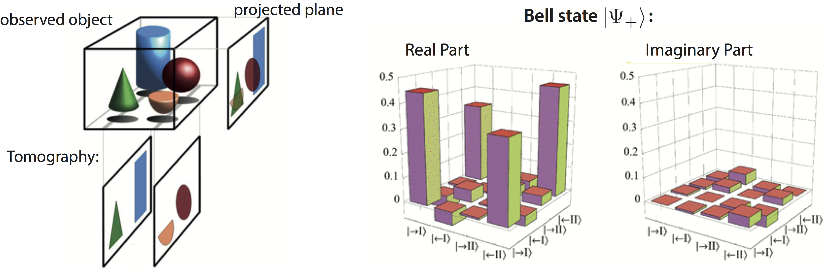
Quantum State Tomography

Quantum state tomography is applied on a source of quantum systems, in order to determine what the quantum state is, that is emitted by the source.  The difference to a usual measurement, that determines the quantum state after a measurement, quantum state tomography aims to to determine the state prior to the (possible) measurement. Sine the quantum state at the beginnings unknown, it is supposed to be a mixed state – so strictly speaking quantum tomography is  fully reconstruction the  density matrix  in a finite Hilbert-space. The general function principal of tomography is schematically illustrated below (left) and an actual reconstructed density matrix of a (neutronic) Bell state ¹ of a single-neutron system having a fidelity of 0.79 is depicted on the right side.

Linear Inversion: The simplest type of Quantum state tomography can be derived simply by applying Born‘s rule, which states that , where  is a particular measurement outcome projector. From a number of measurements an approximation  to  for each  is provided. Next a matrix  is defined as  , with  being a fixed list of individual measurements with binary outcomes. Applying the matrix to a density matrix then yields the following probabilities:  which can be rewritten as . Here    is the representation of the operator  as a row vector and  the representation of the density matrix as a column vector. Linear inversion corresponds to inverting this system using the observed relative frequencies   to derive the vector , which is isomorphic to the density matrix . However, this system is not going to be square in general, as can be seen in the following simple example: a two-dimensional Hilbert space with 3 measurements  and  , where each measurement has 2 outcomes and therefore 2 corresponding projectors which gives 6 projectors in total. But the real dimension of the space of density matrices is (2⋅2²)/2=4, leaving   to be 6 x 4 matrix. To solve this we multiply by   from left which gives  , from which we get  . This will work in general only if the measurement list is tomographically complete. If this is not the case  is not invertible. Another major problem of linear inversion is that the computed solution will not be a valid density matrix, which means that it has negative probabilities or probabilities greater than one for certain measurement outcomes. This typically occurs if only a few measurements are performed. These problems can be overcome by applying different methods:

Maximum Likelihood Estimation: is is one of the most used methods in quantum state tomography. It is a method of estimating the parameters of a statistical model given observations, by finding the parameter values that maximize the likelihood of making the observations given the parameters. By restricting the domain of density matrices to the proper space, and searching for the density matrix which maximizes the likelihood of giving the experimental results. The likelihood of a state is the probability that would be assigned to the observed results had the system been in that state. Assuming the measurements are observed with frequencies of occurrence , then the likelihood associated with a density matrix is expressed as , where is the probability of outcome for the density matrix . Such a procedure incorporates a priori knowledge about relations between elements of the density matrix, which in turn guarantees positivity and normalization of matrix (main problem of linear inversion). Nevertheless, maximum likelihood estimation suffers from some less obvious problems than linear inversion, such as eigenvalues which are 0, this is called rank deficient. This is not physically a problem, since there are states with eigenvalue 0.  This is where the problem arises: it is not logical to conclude with absolute certainty after a finite number of measurements that any eigenvalue  is 0. For example, if a coin is flipped 5 times and each time heads was observed, it does not mean there is 0 probability of getting tails, despite that being the most likely description of the coin.

1. Y. Hasegawa, R. Loidl, G. Badurek, S. Filipp, J. Klepp, and H. Rauch, Physical Review A, 76, 052108 (2007).  ↩

close this window to return to previous page