Experimental Realization: The Three-State-Method

For a general derivation of Ozawa’s generalized error-distitrbance uncertainty relation, expressed as  (see here for details) a non-degenerate meter observable has a spectral decomposition , where varies over eigenvalues of . Then the apparatus A  has a family of operators, called the measurement operators, acting on and defined as . Hence, the error is given by . If are mutually orthogonal projection operators sum and norm can be exchanged and the error can be written in compact form as , where is the output operator given as . The disturbance can be written as .

For an experimental demonstration of the new uncertainty relations from error  and disturbance  have to evaluated experimentally. Though these two quantities were  considered as experimentally unaccessible, to occurrence of the term [ ] when evaluating error [disturbance], Ozawa could overcome this hurdle by proposing the so-called three-state-method ¹: applying the operator identity measurement error and disturbance are given by 
where represents the modified output operator, given by . Consequently error and disturbance can be expressed as a sum of expectation values in three input states , , and , , , respectively. In the case of qubit measurements, as it is the case for the neutron’s spun, the apparatus A has two output ports denoted as (+) and (-), which is schematically illustrated below.

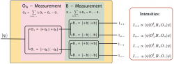
The expectation values of [ ] necessary for the determination of error [ disturbance ], are derived from the intensities at the four possible output ports denoted as and . The expectation value is obtained from the following combination of count rates . As already mentioned due to the prior measurement of the operator measured by a second arraratus A’ is modified from to , with the corresponding expectation value expressed as , required to determine the disturbance . Consequently all expectation values necessary to determine error and disturbance can be derived.

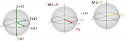
In our experiment the following observables were chosen:  and  . Consequently the three required states for  are i) =   ii)   and . From these three states the error  is determined. In the same manner for  we get the three states  and , which are required to determine the disturbance . A Bloch sphere representation of the required states, and the two the observables  and  is given above.

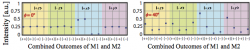
Instead of measuring precisely in direction of   with M1, which would disturb the subsequent   measurement  in M2 maximally an approximate measurement of   , denoted as  is performed instead. The experimentally controlled tuning parameter of  in our case is the azimuthal angle on the equatorial plane of the Bloch sphere. Typical recorded intensities, in the three states, are plotted below for two selected values of above. From these intensities and    are calculated (left):

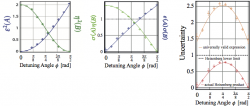
If these results are combined wit the measured standard deviations and (middle) all term occurring on the left hand side of Ozawa’s generalized error-distitrbance uncertainty expressed as  can be determined experimentally.

Alternative Approach: The Two-State-Method

Another possible way to solve the problem from above is to the following operator identity: and again the same for . Then error and disturbance are given by

.
Consequently error and disturbance are again represented by a sum of expectation values in two input states and , being the projections onto the eigenstates of and (multiplied by a factor 2). Note that in this method, referred to as two-state method, the initial state is actually never sent onto the apparatus. The effect of the initial state on error and disturbance manifests here via the auxiliary states and .

back to Experimental Demonstration of generalized Error-Disturbance Uncertainty Relations