Dynamical Theory of Diffraction

In the framework of the dynamical theory of diffraction there are two problems to be solved: The first is to find the conditions under which a wave field can exist in, and travel through, the crystal, which is an extension of optical theory of dispersion. The second problem is that of connecting the fields inside the crystal to those outside, which includes also the incident wave – the answer is the  theory of refraction and reflection.

Contents:

Single crystal plate
Intensities behind the crystal
Borrmann Triangle
The complete (empty) interferometer
Interferometer with phase-shifter
Measurable intensities

Compared to the geometrical theory, the dynamical theory of diffraction accounts for the spatial periodicity of the interaction potential in perfect single crystals. Thereby the Schrödinger equation has to be solved taking this potential into account ^{3 4}. When neutrons illuminate a perfect crystal under near-Bragg orientation conditions, the dynamical theory of diffraction predicts a coherent splitting of the incident wave into four components, with two travelling wave components passing within the crystal in the Bragg direction and two components in the forward (incident) direction. P. Ewald has shown in his historic investigation of the dynamical theory of X-ray diffraction, which in turn characterizes neutron diffraction as well, that this splitting will result in a periodic beating of radiation density travelling in either the Bragg or forward direction at different depths in the crystal, this feature being described as a Pendellösung structure.

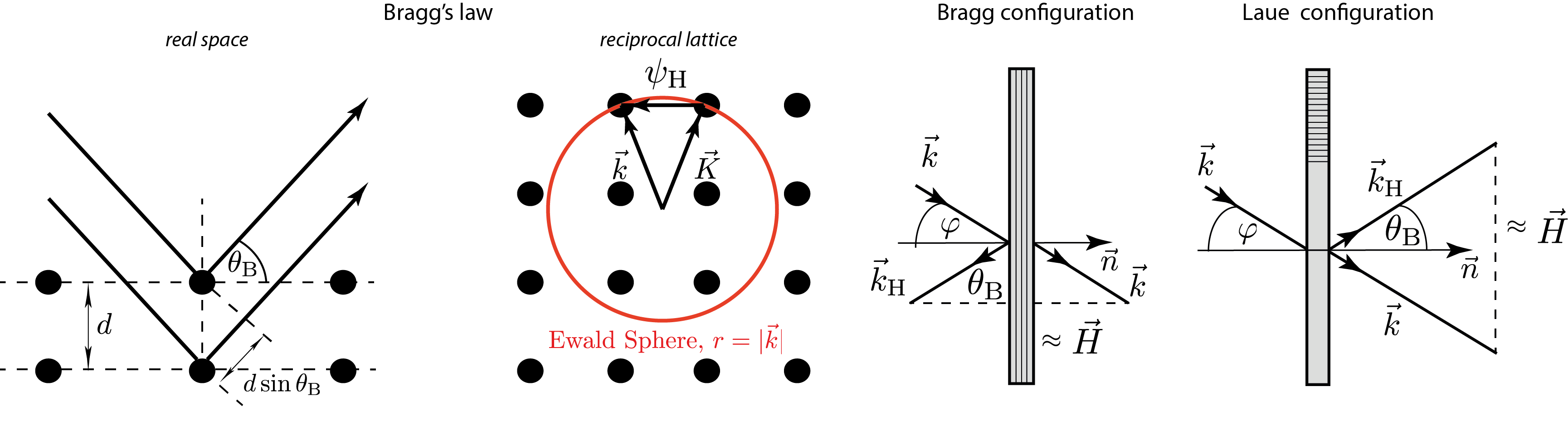
Generally a crystal is made up of atoms arrange in a three dimensional periodic structure, describes by the linearly independent vectors and . If we move in the crystal along a linear combination we arrive at a point with similar surroundings compared to the point before the lineare translation . If we now remove all atoms and only keep the mathematical (point like) structure the result is the Bravais lattice. In addition to the (direct) Bravais lattice described by the basis vectors  a reciprocal lattice with lattice vector , where are the Miller indices, and basis vectors , and with being the volume of elementary cell given by . In the reciprocal lattice the Bragg condition reads , where  denotes the incoming (or outgoing) and  the refracted wavefront, respectively, which is illustrated schematically below on the right side, in comparison with the usual formulation of Bragg’s law , illustrated  in the middle. The general difference between Laue and Bragg configuration is illustrated below on the right.

Single crystal plate: The neutron wave function inside the silicon perfect crystal is deduced by solving the stationary Schrödinger equation for the time-independent crystal potential denoted as , where the potential is given by the sum over all nuclear scattering centres located at and with being the mass of the neutron. See here for crystallographical details of the silicon diamond lattice. The vector of lattice position is given by , where   denotes the vector from origin to elementary cell and   is the vector from origin of elementary cell  to position of atom in cell expressed as . Here   are the lattice vectors of an elementary cell and are rational numbers between 0 and 1. Since the crystal potential is periodic it can be transformed into reciprocal space by calculating the Fourier transformation of the crystal potential as follows: , where denotes the lattice factor and the structure factor.

The lattice factor is given by , where Number of elementary cells and is a reciprocal lattice vectors with , where are the Miller indices, where , and with being the volume of elementary cell given by .

The structure factor is calculated using the definition and as . As a simple example, we consider a body-centered cubic crystal system, with and which yields . Now we consider the (2,2,0)-reflexion of the face-centered cubic lattice of a silicon single crystal, which is (is explained above in detail) of diamond lattice type. Then for (e.g. silicon in -direction) and for all odd/even (e.g. silicon in -direction).

Thus we get . If is the number of scattering centers (or atoms) per elementary cell, then is the number of scattering centers per unit volume. Calculating , the structure factor is always equal to and we get   and . Plugging in the numbers from the table below

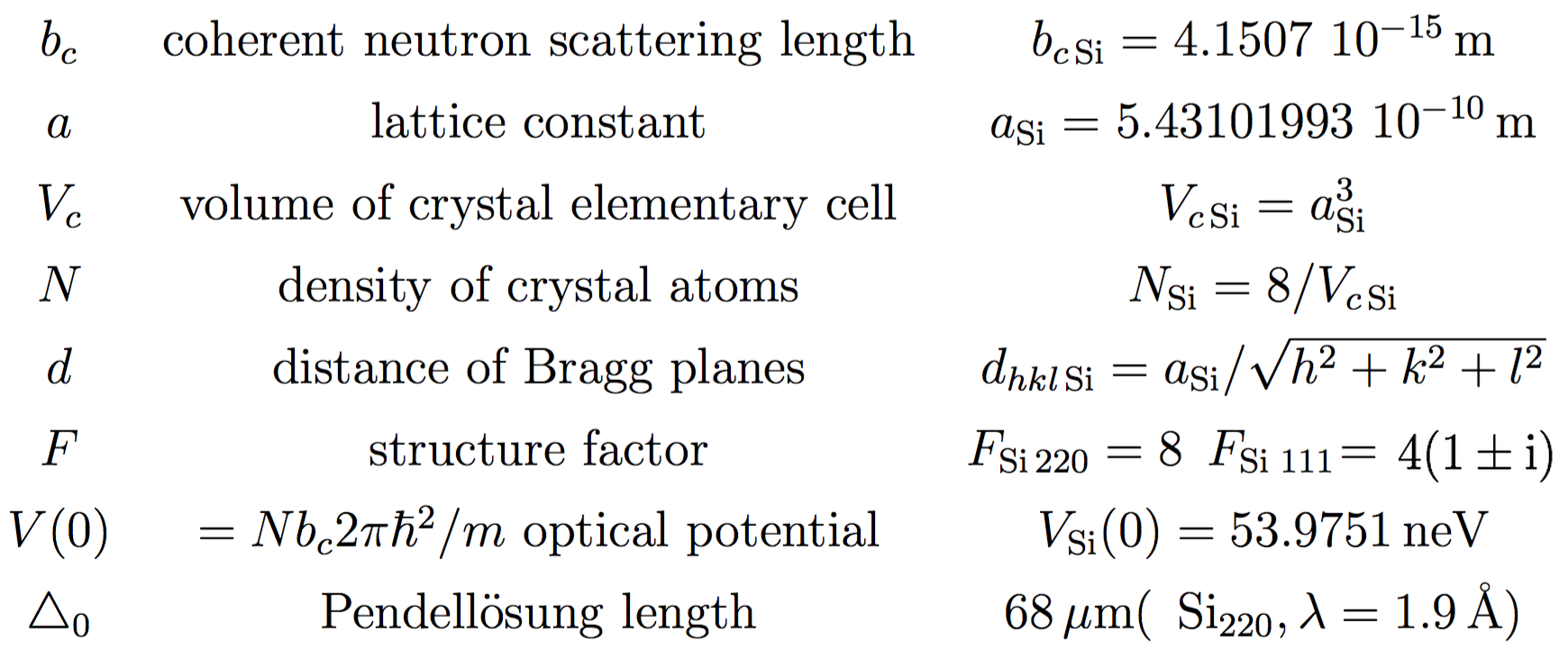
we get eV. For thermal neutrons with energy of about eV the ratio between the potential and the energy yields .  The inverse Fourier transformation of the potential is given by , which describes the periodicity of the potential in the crystal lattice.

Basic equations: Using the so-called Bloch ansatz , where is a wave vector inside the crystal and is the amplitude denoted (in analogy to the potential) as . Hence, the amplitude , which is defined in the reciprocal space, has to be determined. The wave-function is now given by . The basic equations of the dynamical theory of diffraction are therefore given by – a infinite set of coupled equations for the amplitudes , representing equivalent waves in the crystal whose wave vectors differ by respectively. This system of equations cannot be solved generally, nevertheless, the respective amplitudes are expected to be large, if the wave vector of the reflected beam is near a reciprocal lattice point.

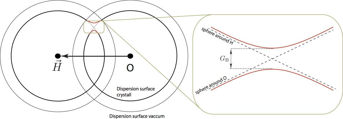
One-beam approximation (beam refraction): Here only the contribution is considered, This approximation is valid, if no Bragg condition is fulfilled. The beam passes through as if the material was non-crystalline. The reflected beam can safely be neglected if the optical potential is small compared to the kinetic energy of the incident neutron. A schematic illustration is given below. In the case of is given by the number of scattering centers in the elementary cell (no periodic structures are taken into account). Since is the number of elementary cells per volume unit, is given by . For a thermal beam with a wavelength of Å the kinetic energy is meV (m/s), which is orders of magnitude larger than typical values of , for example for silicon neV. Thus the corresponding equation is given by , with and . According to the energy conservation, for the free neutron with momentum , of magnitude , the kinetic energy is given by . Hence , since one can write , which yields . In analogy to light optics the refractive index is defined as . In general the wave vector changes both direction and magnitude – the neutron wave is refracted, which is depicted in the illustration below on the left side. Note, that for most materials () this leads to a refractive index slightly smaller than one. However, the neutron index of refraction is typically very close to one, e.g. for silicon . Despite the additional (repulsive) potential the kinetic energy is lowered. The one-beam approximation is valid for a perfect crystal far off any Bragg condition, as well as for homogeneous non-crystalline media. The direction of the beam is calculated according to the continuity of the tangential component , where we get for the perpendicular component we get . Using , where is the surface normal, this can be written as .

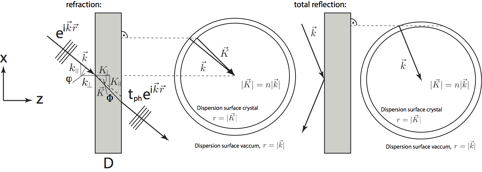
The so-called dispersive surface is an area of constant energy in reciprocal space of radius in vacuum and radius  inside the crystal. The continuity of the tangential component has to be considered inside the crystal t which is the reason for total reflection, which is illustrated above (right).

Two-beam approximation: In this case the beam fulfills a single Bragg condition. Two lattice points have to be taken into account, namely , representing the forward direction, and one single , representing the diffracted direction. This approximation is justified only if all the other lattice points are far away from Bragg refraction. We shall see that the refracted intensity decreases very quickly in close to a lattice point. Hence, from the basic equations from above can be concluded that two equations have to be solved simultaneously:

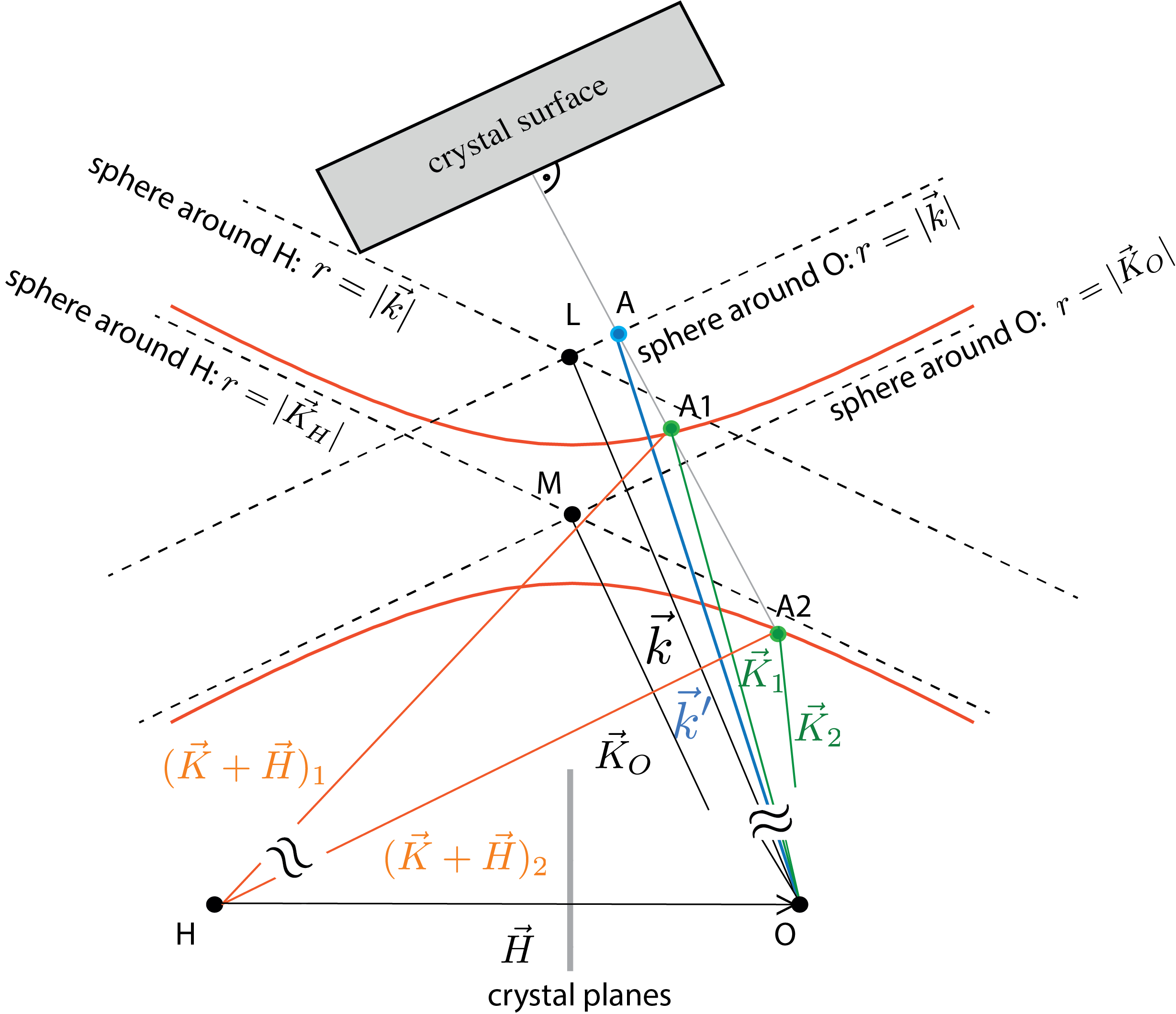
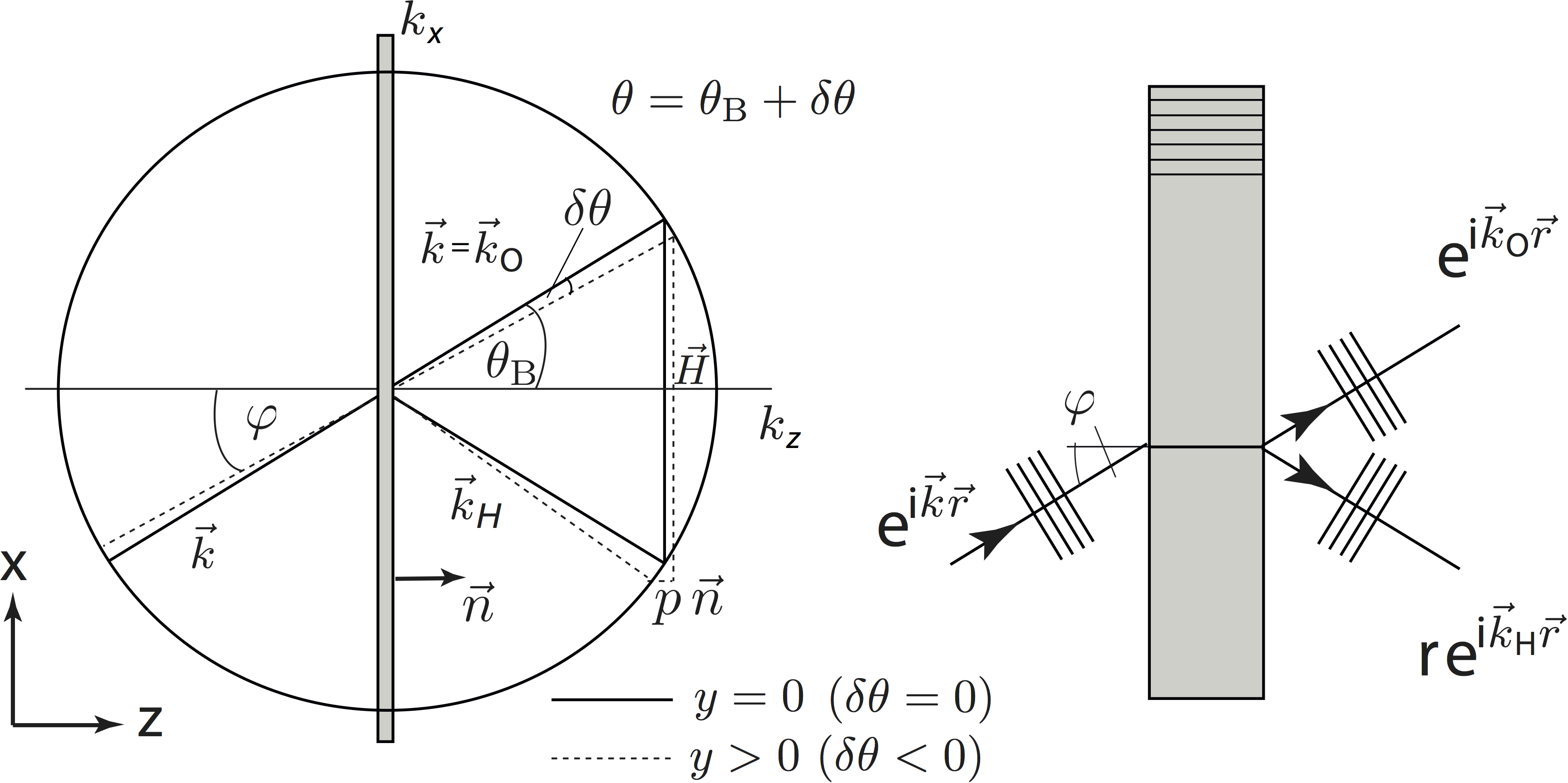
As we have seen in the one-beam approximation in the mean crystal potential is almost equal . Thus we now expect and also to be close to . Consequently we can make the following ansatz: and , where and are introduced as excitation errors, which are in the range of . The vectors themselves are given by for the forward beam and for the diffracted beam, which is depicted in the schematic illustration above. Note that here only occurs, but  and  are not independent due to , which gives , with and . Here characterizes geometrical proportions – Laue diffraction or Bragg diffraction and  describes the deviation from the exact Bragg angle  and therefore defined as .

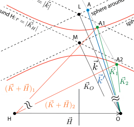
Close to a Bragg condition two reciprocal lattice points lie near the Ewald sphere and therefore two amplitudes of the system of coupled equations, have to be taken into account, which is illustrated above. The separation between the two branches of the dispersion surface is a characteristic inverse length given by .

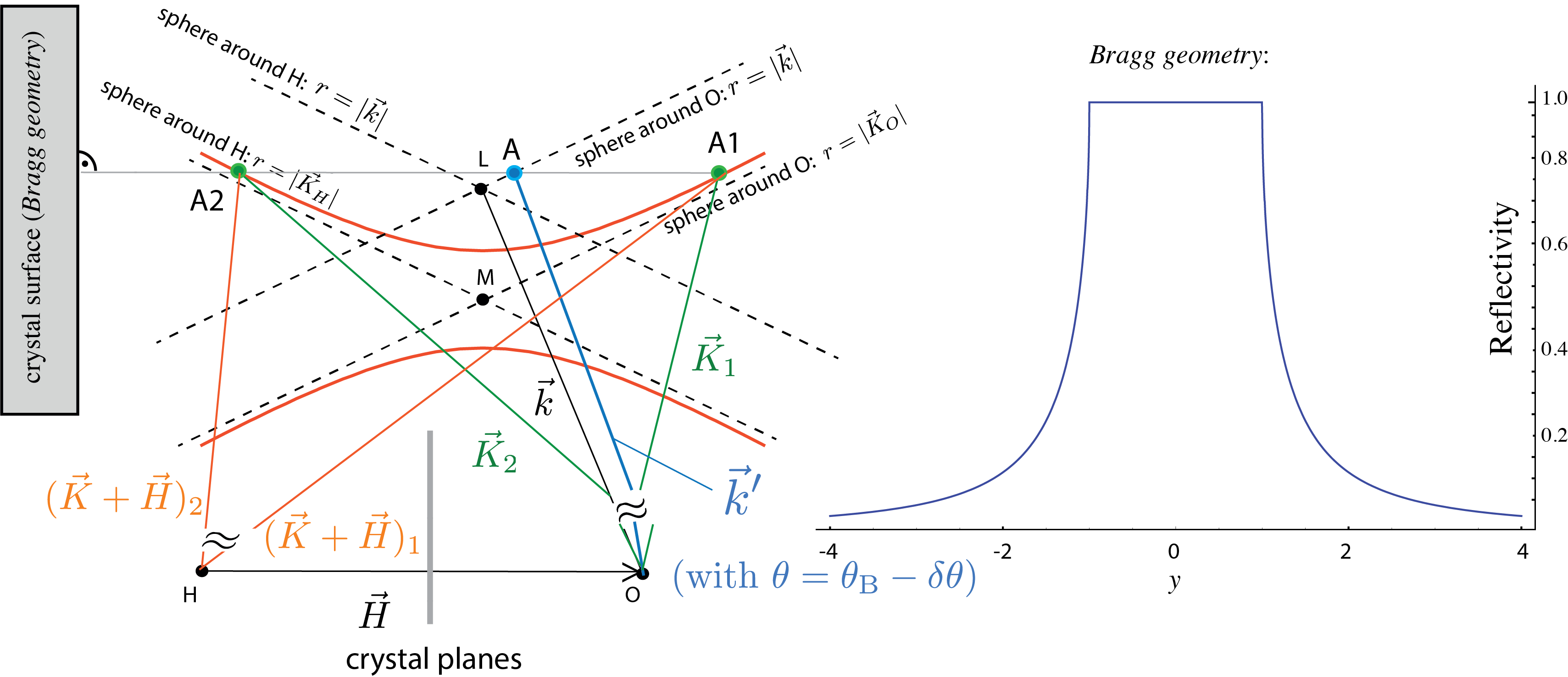
Bragg configuration – the reflection planes are parallel to the crystal surface ()  with  , which gives . Note that the reflectivity close to a lattice point in Bragg geometry is expressed as , which accounts for total reflection. The parameter is a dimensionless parameterization of the deviation from the Bragg angle given by . A graphical illustration on the Ewald sphere is given below. The region with is referred to as Darwin Plateau (or Width) of the crystal.

Returning to the basic equations of the two-beam approximation, we insert these results and obtain the following homogenous equation system:

from which we get , which is called dispersion relation (we only get non-trivial solutions if the determinant is equal to zero). Finally, we get a quadratic equation for expressed as , having the solutions . In the Laue case the solutions read , since ,  and  for the silicon (2,2,0) reflection. Due to the two possible values we have two wave fields in the forward direction as well as two wave fields in the diffracted direction inside the crystal. An illustration of the probability distribution associated with the two wave fields, and given by , is given below on the right side. For wave field the highes probability is found at the position of the Si atoms, whereas for  the maximum of the probability distribution is located between the atoms.  Now we can define the ratio of the amplitudes . The corresponding wave vectors are given by in forward direction and in H-direction, which is illustrated below on the dispersion surface. Hence, two wave functions arise, which are superpositions of the forward and diffracted directions themselves. However, the most interesting are the wave functions that are outside in the forward (O) and diffracted (H) direction given by

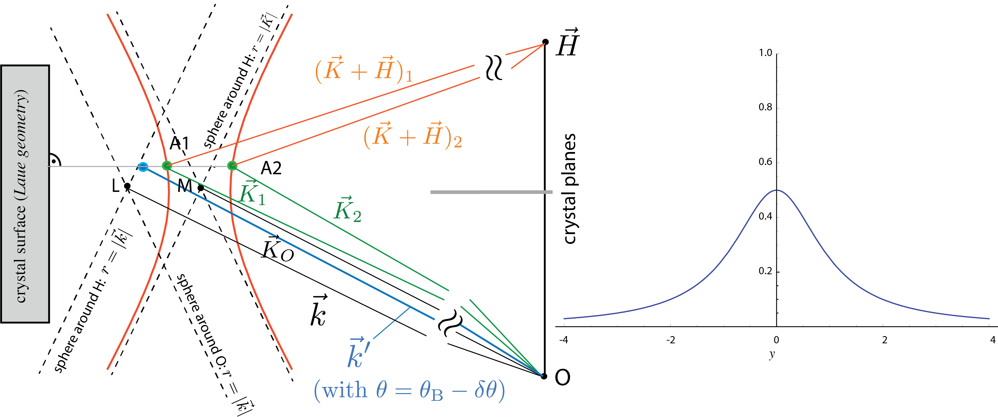
Laue configuration – here, the beam  is diffracted behind the crystal, the reflection planes are perpendicular to the crystal surface (). Furthermore we have , which yields . Hence we get with , where describes the deviation from the exact Bragg angle , that is . Hence, within the framework of the dynamical theory of diffraction, the exact Bragg equation is denoted as , with all these vectors belong to the interior of the crystal. In usual notation a Bragg reflection is obtained when the Bragg condition is fulfilled, i.e.,  with being the lattice plane distance defined the miller indices () and the lattice constant . The thermal neutron wave length is typically in the range of 1.9 to 2.7 Å, which corresponds to energies of 22 to 11 meV and Bragg angles of 30 to 45 degrees for silicon (220)-net plane reflection (m).

Now we have to take a look at the boundary conditions. Putting the coordinate origin on the crystal surface and the -axis parallel to , provides the first boundary condition of the front side of the plate, and (Laue case) accounts for the boundary condition on the back side, where denotes the thickness of the crystal plate. For stake of simplicity the incoming wave is represented by a plane wave written as . The continuity condition of the wave function and the wave function at the front side of the crystal yields . Since there is no reflected wave at the front side in the Laue-case we get as second boundary condition . Combining these equation yields and . The forward and diffracted beam behind the crystal are therefore given by

where and are complex crystal functions, accounting for transmission and reflection.

For the Bragg-case the second boundary condition is that there is no refracted beam at the back side of the crystal. Consequently we get , which yields and . From that we can calculate the forward and diffracted beam intensities in respect to the incoming beam as

Intensities behind the crystal: The squared absolute values and are of interest because they are the ratios of intensity, which are diffracted behind the crystal. Before that, we will introduce new variables to rewrite the expression for , namely  and , which yields . Here the + sign accounts for >, i.e., Laue-case and the – sign for <, that is Bragg-case.

Focusing on the Laue-case we will now calculate the forward and diffracted beam behind the crystal. Here, the parameter is proportional to the crystal thickness with and is referred to as Pendellösung length, simply because the intensity oscillates between the forward and diffracted directions, depending on the crystal thickness , if the Bragg condition is perfectly fulfilled (). Now the parameter can be rewritten as . The absolute value of the wave vector is given by . Note that this is only correct for the special silicon (2,2,0)-reflection, where we have (since ).

The reflected wave vector (inside the crystal) is given by , where the direction of the diffracted beam behind the crystal occurs, which is , with , a correction vector perpendicular to the surface. In addition, we introduce the quantity , which will be used for the wave functions in O and H direction. In forward (O) direction we have , being the incoming wave and with . For the reflected direction we get , which can be further evaluated as with , the quantity denotes the back of the crystal. Note that the index O here denote that initial direction of the the wave front is the O-direction, and and denotes whether it is reflected or transmitted. The intensities in respect to the incoming wave behind a single crystal plate are expressed as

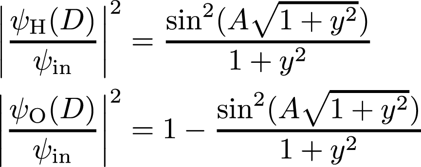
Before we analyze this equations in more detail we will take a look at a optimal arrangement (no deviation fromm the Bragg angle), which means that . The behavior of the intensities in forward (O)- and H- direction as a function of the thickness is plotted below.

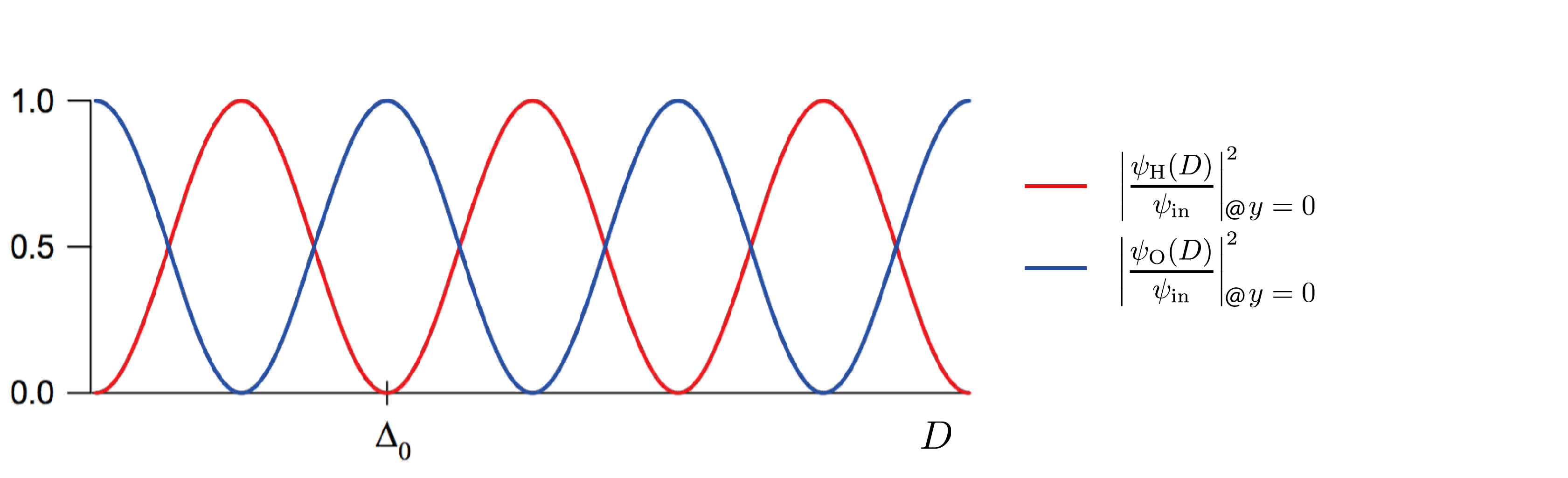
The intensity also oscillates as a function of the deviation from the Bragg angle and these oscillations become narrower the thicker the crystal is. The intensities, dependent of the deviation from the Bragg angle for the O-beam on the left and the H-beam on the right for different thicknesses  of the crystal plate, are plotted below.

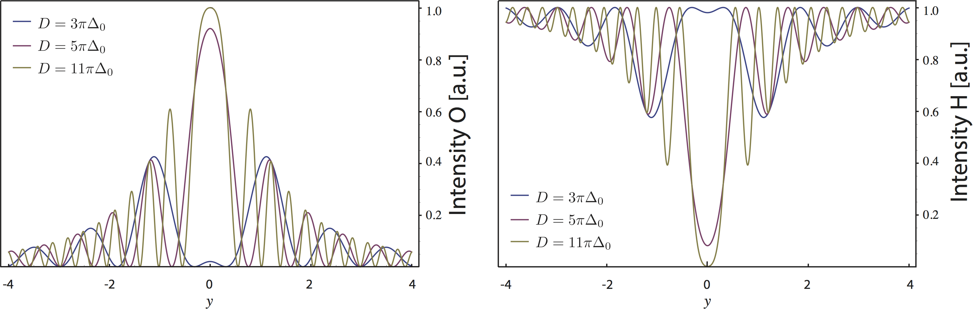
For a silicon crystal of thickness mm and thermal neutrons of a wavelength Å the spacing between two intensity minima is less than 5 seconds of arc, which due to facts like beam divergence and wavelength distribution cannot be experimentally resolved any more. Consequently for realistic crystal thicknesses, i.e., we can average the function . So from that we get the reflection curve for a thick crystal in Laue configuration , which is illustrated a few lines below on the left side. As can be seen in the diagram the maximum of the reflection curve is 1/2. The width at half maximum is , which in terms of angles reads , which for the silicon 220-reflex and thermal neutrons of a wavelength Å is roughly 1.2 seconds of arc.

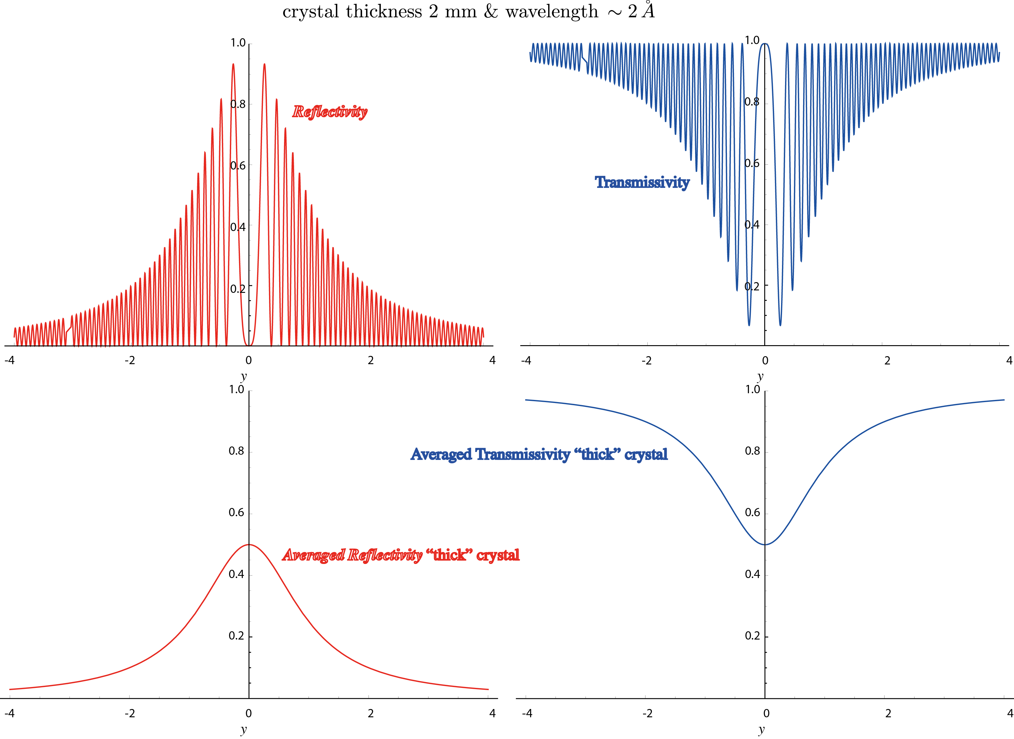
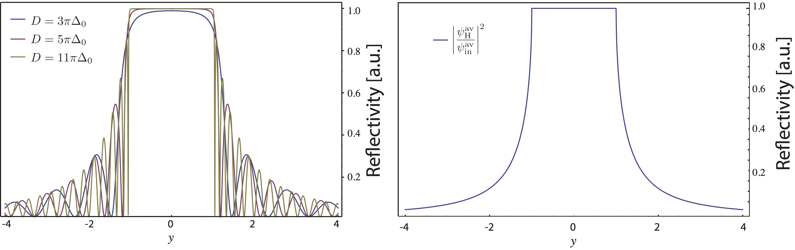
For the Bragg case the situation is different: As we have already seen in the discussion of the dispersion surface, for the Bragg configuration there exists a region of total reflection. This region having is referred to as Darwin Plateau (or Width) of the crystal. The respective intensities are given by

From that we get after averaging for  and for , which is illustrated below on the left side. On the right side the averaged intensity is plotted.

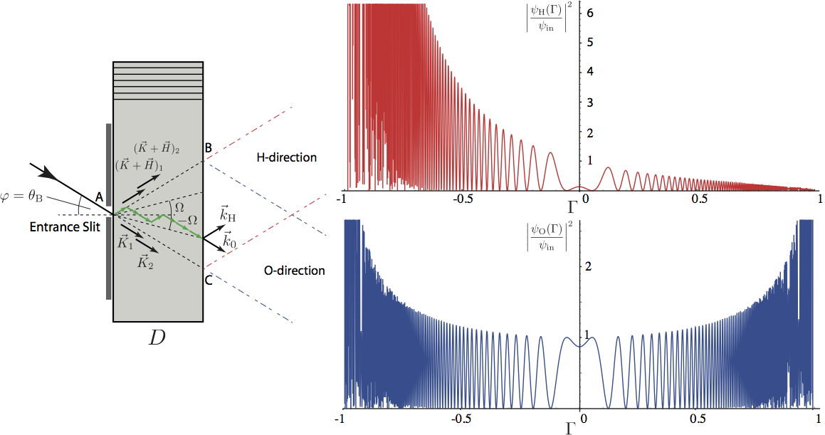
Borrmann Triangle: Before we can calculate the flow of particles emitted from the crystal under an angle from the crystal planes, it is useful to define a dimensionless parameter as

Again focussing on the Laue-case () we get , where – and + denote wakefield 1 and 2, respectively. From that we can conclude that the angle for the particle flow in direction  as a function of   varies between 0 and the Bragg angle. Thus even for a small beam divergence  (e.g. 1 minute of arc) we have excitation of the entire Bormann triangle ABC.  The corresponding intensities, as a function of   are given by

which is illustrated below for a crystal of thickness mm. At first sight is seems it seems surprisingly that the intensity is not maximal at , where the Bragg condition is fulfilled exactly. This is due to that fact that the outer regions correspond to larger intervals of the incoming neutron beam.

The complete (empty) interferometer: Since all our interferometers are of triple Laue (LLL) type (or even LLLL) from this point on we only discuss Laue configurations (The Bragg is only discussed up the point of a single crystal plate, because this is used for instance for the monochromator). If we apply the calculations from above ( and to the second and third interferometer blade, the incident wave may also be in direction, which is depicted here:

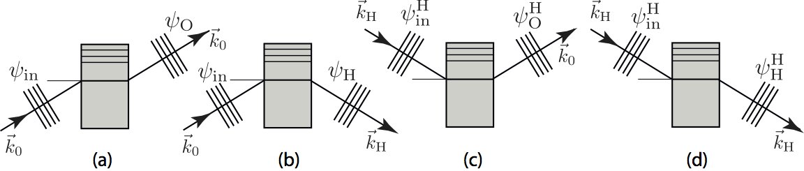
, , , with and finally . Thus we distinguish waves have direction O and H instead of reflected and transmitted – to sum up:

By applying these to the second and third interferometer plate all wave functions of the LLL interferometer depicted below can be calculated. Note that factors and also depend the crystal thickness  , as well as on the position of the crystal plate’s back. For the general case we assume different thicknesses for each blade and we them with the subscripts  for beam Splitter, Mirrow and Analyzer. We start with beam path I, where we get behind the beam splitter S , and behind the mirror M . Behind the beam analyzer A we have  and . All together the wavefunctions of beam path I are given by  and . Likewise we can calculate the wavefunctions in beam path II, where we get behind the beam splitter S , and behind the mirror M . Behind the beam analyzer A the wavefunctions read   and . All together we get  and .

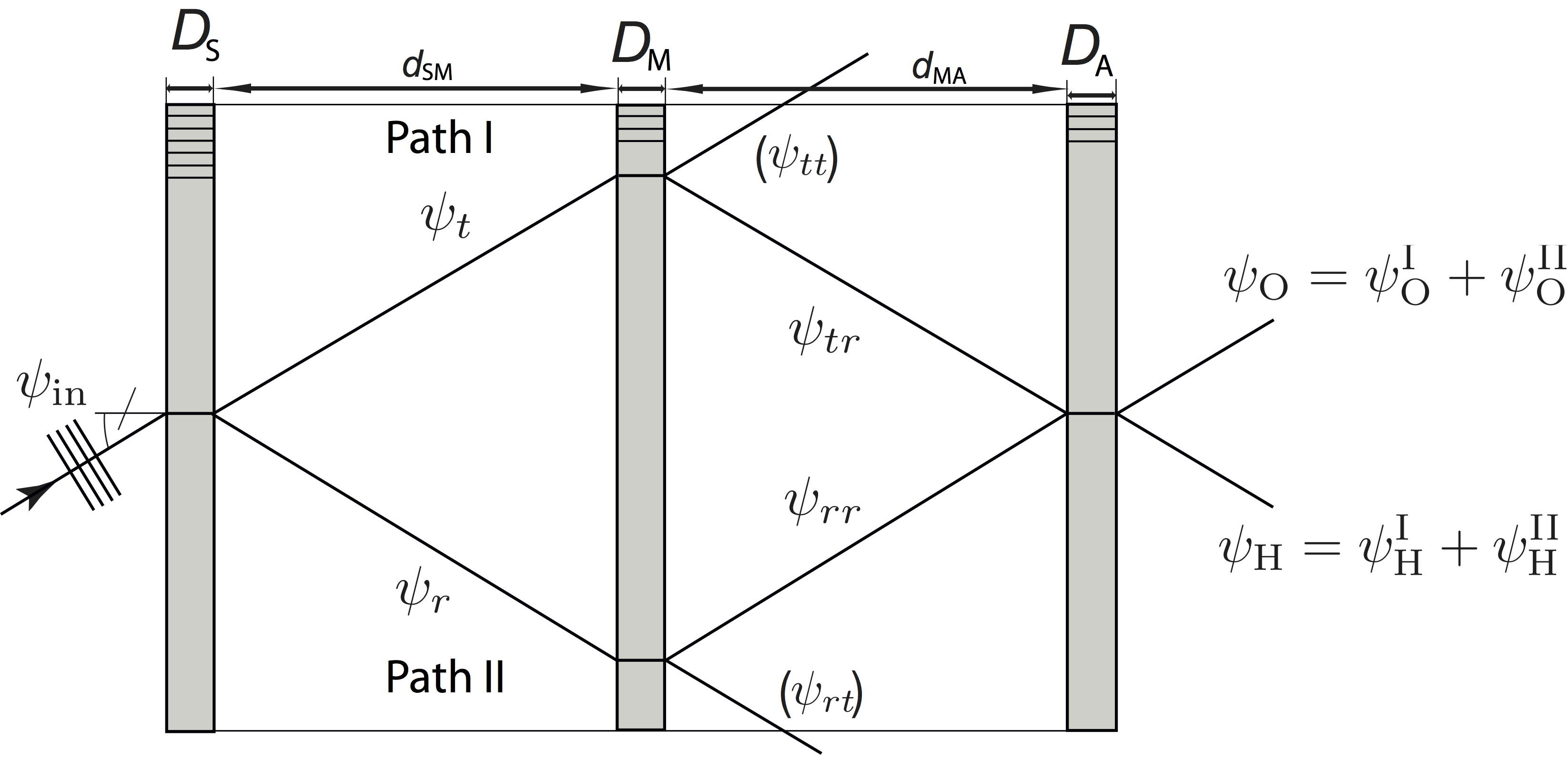
Thus, the focusing condition for an ideally perfect interferometer is given by , which just means that the three plates of the interferometer have to be equal and they have to be equispaced. Consequently in the forward direction, the two wavefunctions are equal expressed as  . Both wave functions are reflected twice and transmitted once (rrt). Both wavefunctions  have equal amplitudes and equal phases, which is the most important result concerning the perfect Laue interferometer. The final wavefunctions in the O and H beam are the superpositions of both path contributions:

Finally, the last step is to compute the intensities in O and H beam in respect to the incoming wave, which yields

In the next step we will average of the Pendellösung oscillations. This is justified since they oscillate at a frequency that practically cannot be resolved any more, as discussed above. Furthermore it should be mentioned, that in practice a neutron beam has a finite spectral width, which is also large compared to the the structure of the Pendellösung oscillations. Finally we get for the average intensities and , which is illustrated below.

It can clearly be seen, that in forward (O) direction we have a maximum for prefect orientation (), whereas in H-direction we find a (local) minimum, as a consequence of the -phase shift between the two ongoing beams. Note that this -phase shift relations is independent of . Since 50 per cent of the initial intensity are lost at the second plate a maximum of 0.5 is reached for  at .

Interferometer with phase-shifter: as seen before the phase difference between the sub-beam belonging to path I and II is zero for forward (O)-direction and  in H-direction. If we now insert a phase-shifter plate in one of the two beam paths (either I or II) the phase relation between the two sub-beams can be altered, which is illustrated below on the left side. The respective image shows a phase-shifter plate in beam path I of thickness  having a mean index of refraction of  given by . According to the one-beam approximation (see here) the wave vector inside the phase-shifter is (see here). Since the surface of our phase-shifter is perpendicular to the incoming neutron beam we get . Now we can calculate the phase shift induced by a phase shifter of thickness as . So all we need to do is to replace the wave function from path one of the empty interferometer with the one including the respective phase-shift: . The phase shift can be rewritten as , where we introduced the quantity , which is the thickness of a phase-shifter causing a phase shift, and is expressed as . Hence we get for the intensity in forward (O)-direction . Since that for a non-absorbing phase-shifter the total intensity remains unchanged, i.e., we get for the intensity in H-direction .

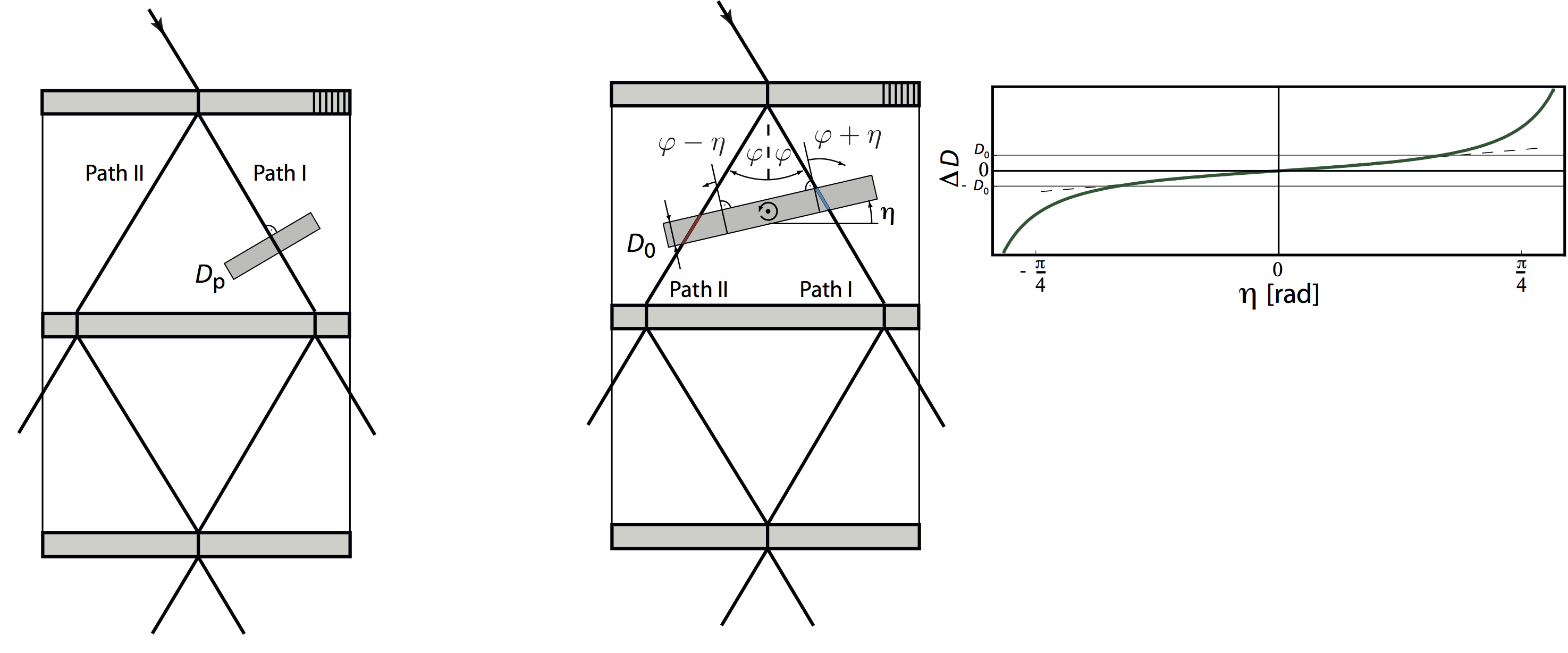
Next we will analyze the situation where the phase-shifter covers both beams.  The thickness of the slab, more precisely the relative path length, now  changes differently for the two partial beams, depending on the angle , as indicated by the red and blue line in the schematic illustration above. The wave-functions of the empty interferometer are now modified as follows: and . Thus the phase difference is determined by the path difference, which yields , where is the rotation angle of the phase shifter slab. As seen in on the right side the function is almost linear for small . Thus an interferogram recorded versus remains sinusoid essentially. By rotating the plate,  can be varied systematically, yielding a final intensity in forward (O)-direction of .

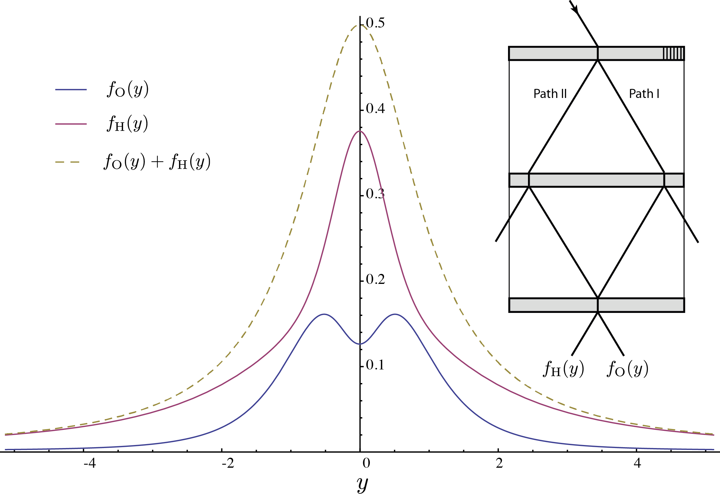
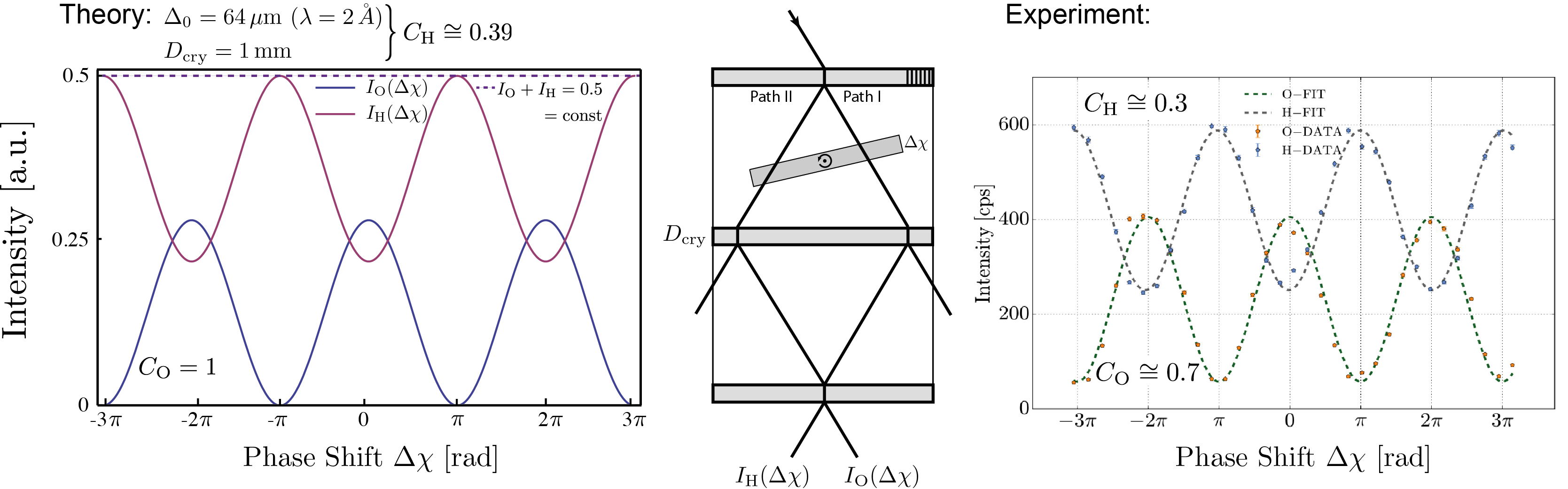
Experimentally measurable intensities:  Since the divergence of the incident beam is much grater than the inherent width of the reflectivity we must integrate the expressions and over , or equivalently over to obtain the experimentally measured intensities which we will denote and , where is an induces phase shift as discussed above. The coefficients, that now still depend on the thickness of the crystal and on the wavelength (via the Pendellösungs length ) are given by and . The measurable intensities are then expressed as

where is the effective beam intensity ( is the amplitude of the incident wave), as in Basic Concept & History of neutron interferometry. For the 220 Si reflection with wavelength Å (Pendellösung length m) and a crystal thickness of 1mm () the resulting of a numerical evaluations yield and . From that we immediately see that we can have a contrast of 100 per cent in the O-beam, while the contrast in the H-beam is limited by 39 per cent, which is illustrated below on the left side (Theory). On the right side a typical (actual) measured interferogram is depicted, where the contrast in the O-beam reaches value of 0.7, which is already considered as a high-contrast measurement.

At this point we want to draw your attention to the book Neutron Interferometry: Lessons in Experimental Quantum Mechanics, by Helmut Rauch and Samuel A. Werner ², which includes more than 40 neutron interferometry experiments along with their theoretical motivations and explanations.

1. H. Rauch, W. Treimer, and U. Bonse, Phys. Lett. 47A, 369-371 (1974). ↩

2. H. Rauch and S.A. Werner, Neutron Interferometry, Clarendon Press Oxford (2000). ↩

3. H. Rauch and D. Petrascheck, Grundlagen für ein Laue Neutroneninterferometer – Teil 1 & 2 (1976).↩

4. M. Suda, Quantum Interferometry in Phase Space, Springer (2006). ↩