Entropic Noise-Disturbance Uncertainty Relations: Experimental Details

State-preparation: In order to prepare the eigenstates of , that is and  (since ) the current through the spin turner coil DC-1 is simply turned off for the former and set to the predetermined  flip current generating the magnetic field for the latter. To prepare the eigenstates of , the respective currents generating the magnetic field  that cause -roations of the Bloch vector, are applied in DC-1. Each of the two eigenstates of and is sent with equal probability.

Measurement of M and B: The projective measurement of consists of two steps. At first, we have to project the initially prepared state onto the eigenstates of , then, in order to complete the measurement, we have to prepare the neutron spin in the eigenstates of . Since the input eigenstates and and the all lie in the -plane of the Bloch sphere, the distance between DC-1 and DC-2 has to be chosen such that the Bloch vector undergoes integer multiples of the full rotation period in their intermediate guide field. Then, spin turner DC-2 rotates the spin component to be measured, which depends on the polar angle (, towards the -direction. For the eigenstate belonging to eigenvalue the component along and for eigenvalue the spin component along is rotated in the -direction. The second supermirror (first analyzer) then selects only the part of the spinor wave function. The projective measurement is completed by the preparation of the measured spin component with spin turner DC-3. In analogous manner to the preparation of the initial state, this is accomplished by properly setting the respective currents in DC-3 required for the fields and . Thus when leaving DC-3 the system is in the appropriate eigenstate of . For the -measurement the same procedure as for the -measurement is applied, that is to rotate the component towards the -direction with DC-4, followed by another supermirror (second analyzer). A further DC coil for preparing the measured spin state can be omitted, since the neutron detection is insensitive to the spin

Noise Determination via Intensities: here we want to explain in detail how the probabilities needed for the calculation of noise and disturbance are obtained from the intensities measured in the experiment. In order to determine the information-theoretic noise, the eigenstates of are sent onto the measurement apparatus which then projectively measures and resulting in four different output intensities for each input eigenstate. We have schematically depicted the measurement process below. The polarimeter setup is adjusted such that it realizes one of the eight possible “arms” of the figure after the other.

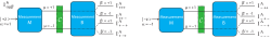
The output intensities get labeled with three lower indices having the values where gives the sign of , indicates which projection operator of has been realized, and does the same for the projection operator of . The probabilities are connected to the intensities via . However, the definition of the information theoretic noise is not in terms of the conditioned probability but , since it quantifies how well the observable’s value can be guessed from the outcome and not contrariwise: . Here is the conditional entropy and and denote the classical random variables associated with input and output . The information-theoretic noise thus quantifies how well the value of can be inferred from the measurement outcome and only vanishes if an absolutely correct guess is possible. Thus, we have to use Bayes’ theorem to connect these different conditional probabilities . The marginal probability is given by summation over of the joint probability distribution where . Now, the information theoretic noise  can be calculated (see here for an introduction to probability theory).

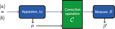
Disturbance Determination via Intensities:  next the eigenstates , that is , of the disturbed observable are sent onto the apparatus. By labeling the output intensities with , which is illustrated below

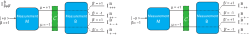
we get the required probabilities from . By again using Bayes theorem we obtain the probabilities as they occur in the definition of the information-theoretic disturbance . In our scenario, the measurement operator is varied over the -plane spanned by  and with  and the theoretically expected expressions for the probabilities are and . Here is used to denote the probabilities in the case that  an optimal correction is applied after the -measurement. These expressions yield , with . These theoretically expected value of noise and disturbance which are depicted in the main text.

Optimal Correction Procedure for projective Qubit Measurements: for a spin measurement operator and an observable the optimal correction minimizing the disturbance after the projective measurement of on is given by

with and being the respective projection operators of . The above formula can be intuitively understood as a sort of maximum likelihood correction procedure: the output of the apparatus is rotated onto the closest eigenvector of , which is , if and are more correlated than anti-correlated (i.e., ), or otherwise (i.e., ). This guarantees that the outcome obtained from the final measurement of is perfectly correlated with the outcome of , if , or perfectly anti-correlated otherwise—in either cases, correlations are kept maximal, by avoiding the occurrence of extra random noise.