Coherent energy manipulation in single-neutron interferometry

Contents:

Jaynes-Cummings Hamiltonian in RF-flip process
Zero-Field Phase

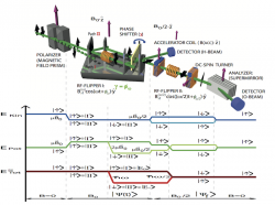
When operating an RF-flipper inside the interferometer, there is a fundamental insufficiency, due to the interaction with a time-dependent magnetic field (see here for details). the total energy is no longer a conserved quantity in RF-flip process. The corresponding wave function is given by , with . After passing the RF-flipper neutrons which were initially polarized parallel to the guide field (-direction), and had the energy , have been flipped and lost an amount of energy . The polarization of this state is not stationary, due to a energy difference of between the spin components: . However, the energy difference between the orthogonal spin states can be compensated by inserting a second RF-flipper, behind the third plate if the interferometer, operating at a frequency of , which is reported in ¹. This flipper evens the energy difference between the two spin components, by absorption (in state ) and emission (in state ) of photons of energy . Hence a combination of two different guide fields, providing the requested static magnetic fields to fulfill the frequency resonance for and , is required. A schematic representation of the setup is depicted below.

close this window to return to previous page

Jaynes-Cummings Hamiltonian in RF-flip process

Concerning a theoretical treatment of the induced RF spin flip the time evolution of the system is described by a photon-neutron state vector, which is an eigenvector of the corresponding modified Jaynes-Cummings (J-C) Hamiltonian ², named after Edwin Thompson Jaynes and Fred Cummings. The J-C Hamiltonian can be adopted for a system consisting of a neutron coupled to a quantized RF-field. Since two RF-fields, operating at frequencies and , are involved in the actual experiment, the modified corresponding J-C Hamiltonian is denoted as

with . The first term accounts for the kinetic energy of the neutron. The second term leads to the usual Zeeman splitting of . The third term adds the photon energy of the oscillating fields of frequencies and , by use of the creation and annihilation operators and . Finally, the last term represents the coupling between photons and the neutron, where represents the mean number of photons with frequencies in the RF-field. Note that the first two and the last terms concern the spatial and the (time-dependent) energy subspaces of neutrons, respectively. The state vectors of the oscillating fields are represented by coherent states , which are eigenstates of and . The eigenvalues of coherent states are complex numbers, so one can write with . The action of on and is given by , and . One can define a total state vector including not only the neutron system , but also the two quantized oscillating magnetic fields: , where for simplicity a single-plane-wave representation for the neutron’s wavefunction is chosen: At this point one can take a look at the action of the interaction Hamiltonian (of one RF-field at frequency ) on a spin-up state:

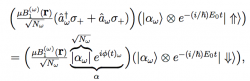
where represents the usual coupling strength of the neutron field interaction which yields after the interaction with RF-field. A spin flip due to emission of a photon of energy and a phase factor from the coherent state of the oscillating field. Now the time evolution of a dressed state, as defined above, is taken into account, to see the effect after passing the RF-field region:

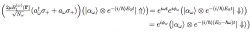
Here is associated with a corresponding state vector , just like in an atomic two-level system, where a certain energy level is associated with a ground state . Hence can be identified with (in analogy to the exited state ). Thus our equation yields

Thus, a third degree of freedom in neutron interferometric has become experimental accessible. See here for experimental demonstration of tripartite entanglement in the single-neutron system.

Zero-Field Phase

Interacting with a time-dependent magnetic field, the total energy of the neutron is no longer conserved after the spin-flip. Photons of energy ω are exchanged with the RF-field, this particular behavior of the neutron is described by the ’dressed-particle’ formalism. Consequently the two sub-beams and now differ in total energy. Therefore the neutron state can be considered to consist of the three subsystems, namely the total energy, path and spin degree of freedom. A coherent superposition of and  results in the multiply entangled dressed ³ state vector, expressed as . According to the notation introduced above we can rewrite this as . The two sub-beams are recombined at the third plate, which is described by the projection operator , resulting in a time-dependent state vector due to the different energies of the two partial wavefunctions. Due to the orthogonality of the energy and spin eigenstates the measured polarization is zero and no intensity modulations are observed in the H-beam, have the following time-dependent polarization . The as well being time-dependent polarization in the O-beam is expressed as , which results in a no-contrast measurement, when the spin is analyzed in -direction, which is illustrated in the animation below.

However, this can be circumvented the following way: The beam recombination is followed by an interaction with the second RF-field, with half frequency . The total state vector is given by

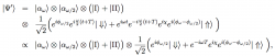
where and are the phases induced by the two RF-fields. The second RF-flipper is operating at half the frequency of the first RF-flipper. By choosing a frequency of for the second RF-flipper, the time-dependence of the state vector is eliminated since both components acquire a phase , depending on the spin orientation. Only a constant phase offset of , which is referred to as zero-field phase, with being the neutron’s propagation time between the centre of the first and second RF-flipper coil, remains in the stationary state vector. Hence the second RF-flipper compensates the energy difference between the two spin components, by absorption and emission of photons of energy .Alternatively this can be seen by applying the operator
on the equation above which yields

The energy difference between the orthogonal spin states is compensated by choosing a frequency of for the second RF-flipper, resulting in a stationary state vector. Hence the time dependence of the polarization vector is eliminated: , with , consisting of the phases induced the path (phase shifter ), spin (phases of the two RF-fields ), and energy manipulation (zero-field phase ). However, the stationary polarization is still lying in the xy[\latex] plane. Here, an addition DC spin-rotator is required, in order to observe an interference pattern, which is illustrated in the animation below.

1. S. Sponar, J. Klepp, R. Loidl, S. Filipp, G. Badurek, Y. Hasegawa, and H. Rauch, Phys. Rev. A 78, 061604R (2008); arXiv:quant-ph/0803.3545. ↩

2. E. T. Jaynes and F. W. Cummings, Proc. IEEE 51, 89 (1963). ↩

3. E. Muskat, D. Dubbers, and O. Schärpf, Phys. Rev. Lett. 58, 2047 (1987). ↩