Asking Neutrons where they have been – Past of a quantum particle

Quantum theory provides the foundation for much of the technology of modern society and is probably the most successful theory unto date. Nevertheless, some aspects remain 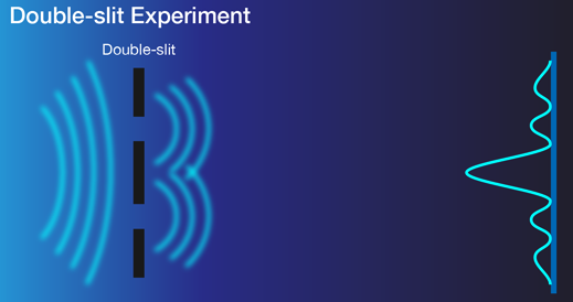unclear even for the experts. One of these is the history of a quantum particle: when we measure a particle in our detector, we lear nothing about the trajectory it took to get there from the source – quantum theory simply has no answer to this question. This is very different from what we experience in our every day life: a classical particle traveling between two points always has a single trajectory as its history (think of a ball for instance). But the history of a quantum particle arriving at a detector is made up of every path it could have taken from where it was emitted. Let’s take a look at the famous double slit experiment, depicted on the left, when interference is observed. On the right we have a double slit experiment aiming to find which path a photon takes by inserting a lens after each slit—the idea being that each lens will only collimate those photons arriving from its respective slit. In this “which-way” measurement the interference will be lost ending up with two distinct spots, one for each slit. Apparently  there is no 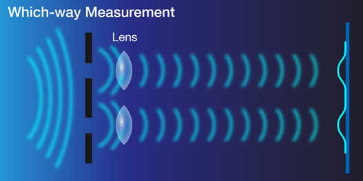confusion in this case: the photon had a single trajectory as its history. Lev Vaidman and his co-workers call even this seemingly safe assertion into question applying the following experimental setup ¹: Danan et al. use a Mach-Zehnder interferometer (MZI) tuned such that theoutputs interfere constructively, ensuring that all photons exit the second beam splitter in the same direction. The authors probe where the Click here (or on the picture) for an animation of a strong neutronic which-way measurement photons were in two situations: i)  interference measurement and ii) when there is a which-way measurement. To label the particular path of the photon, i.e., whether it went via the upper or lower arm, the authors insert in each arm a mirror whose vertical tilt vibrates at a unique frequency. Then, the authors monitor the frequency spectrum of the vertical position of the photons exiting the second 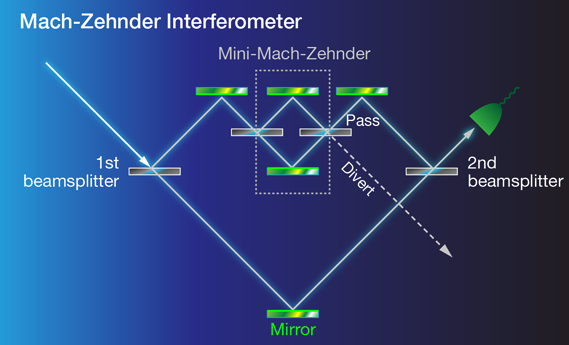beam splitter. If the spectrum contains the same frequency as that of the vibrating mirror in thisuggests some of the photons traveled down that arm. And indeed, i) when the beam splitter that combines light from the upper and lower arms is in place, two frequencies are observed, suggesting photons traveled through both arms. ii) Removing this beam splitter functions as a which-way measurement; only light from the lower arm reaches the detector. In this case Danan et al. only see the frequency associated with the lower arm. Next Danan et al. insert a mini-MZI in the upper arm so that photons pass from the upper arm to the second beam splitter only when the mini-MZI is set for constructive interference, while deconstructive interference diverts this light. In this way, the mini-MZI lets the experimentalists switch between observing interference between light that traveled in the upper and lower arms of the large MZI and observing only that light that traveled through the lower arm. Now all the mirrors vibrate in the upper arm. When the mini-MZI set to pass light i), the researchers observe frequencies corresponding to every path through the system to the detector. That is, the photons had no unique trajectory, much like in the double-slit experiment. But by setting the mini-MZI to divert light exiting the upper arm ii) , the authors again see frequencies from both of the arms inside the mini-MZI, a perplexing observation for two reasons. First, it implies the photons
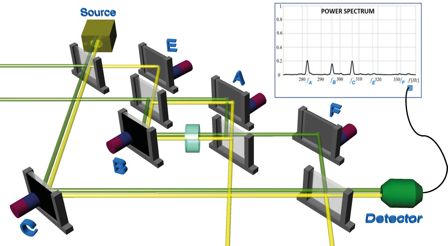reaching the detector traveled down a path (the upper arm) that should never have reached the detector. Second, they don’t see the frequencies from the mirrors just before and after the mini-MZI in the upper arm, so it’s as though the photons in the upper arm passed through the mini-MZI but never entered or exited it. So the authors suggest discontinues trajectories of their photons. Danan et al. argue that this can be intuitively understood: one should consider not just the possible paths of the photons traveling forwards through the system but also the paths that a photo traveling backwards from the detector could take, an idea captured by what is called the two-state vector formalism ². The locations where these forwards and backwards paths coincide will have its corresponding frequency appear in the detected spectrum which is illustrated on the right side. However, the experiment was carried out with a classical laser beam and their results can be fully explained within the framework of Maxwell theory. To test the statement of Danan et al. an experiment of pure quantum nature is called for, which we have done in our neutron interferometric experiment ³, which is schematically illustrated below.

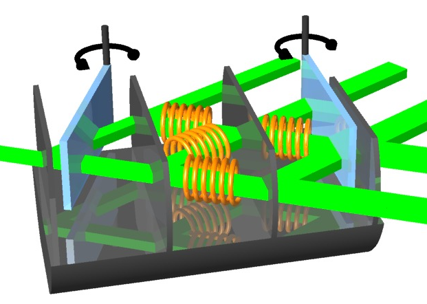
At this point let us switch back to neutrons. A usual or strong which-way measurement is implemented by inserting a detector in one of the beam path. This procedure is illustrated by the animation below.

In our neutron interferometric experiment the energy degree of freedom of neutrons is utilized to weakly mark the neutron’s paths in a three-beam interferometer (IFM). A monochromatic neutron beam enters the IFM consiting of four plates, each working as a 50:50 beam splitter.

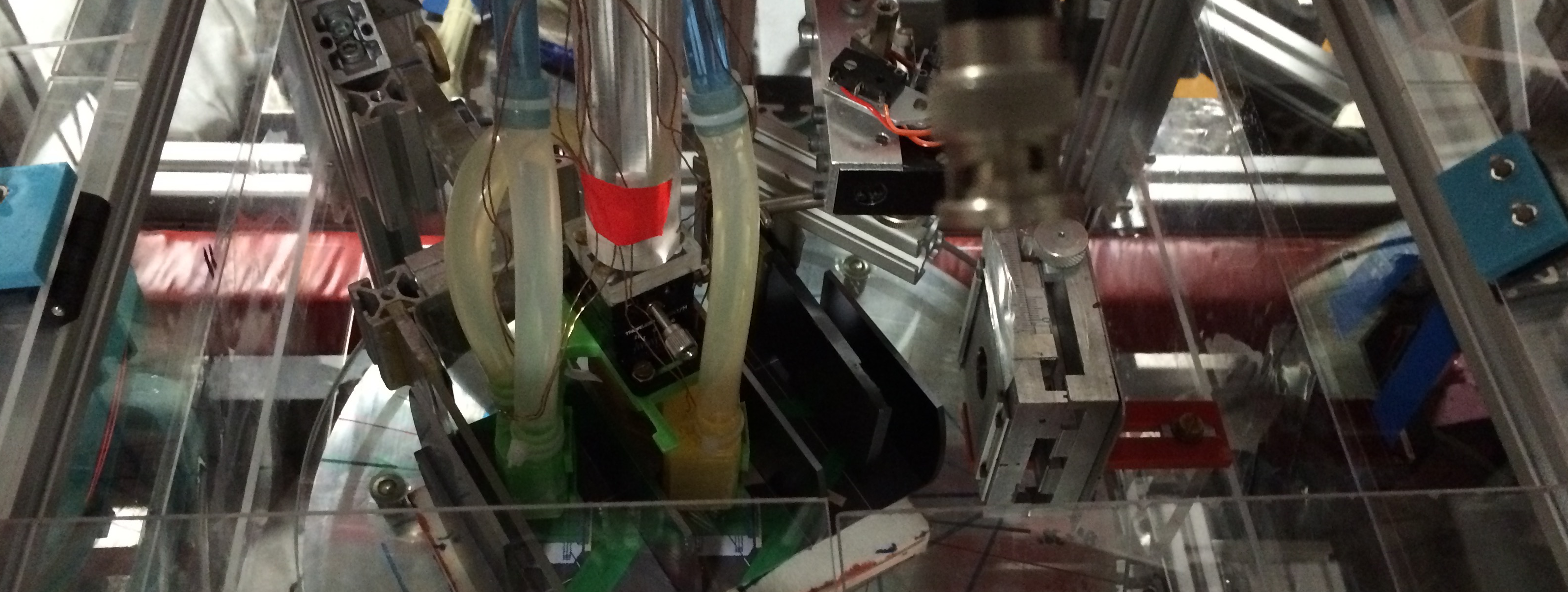
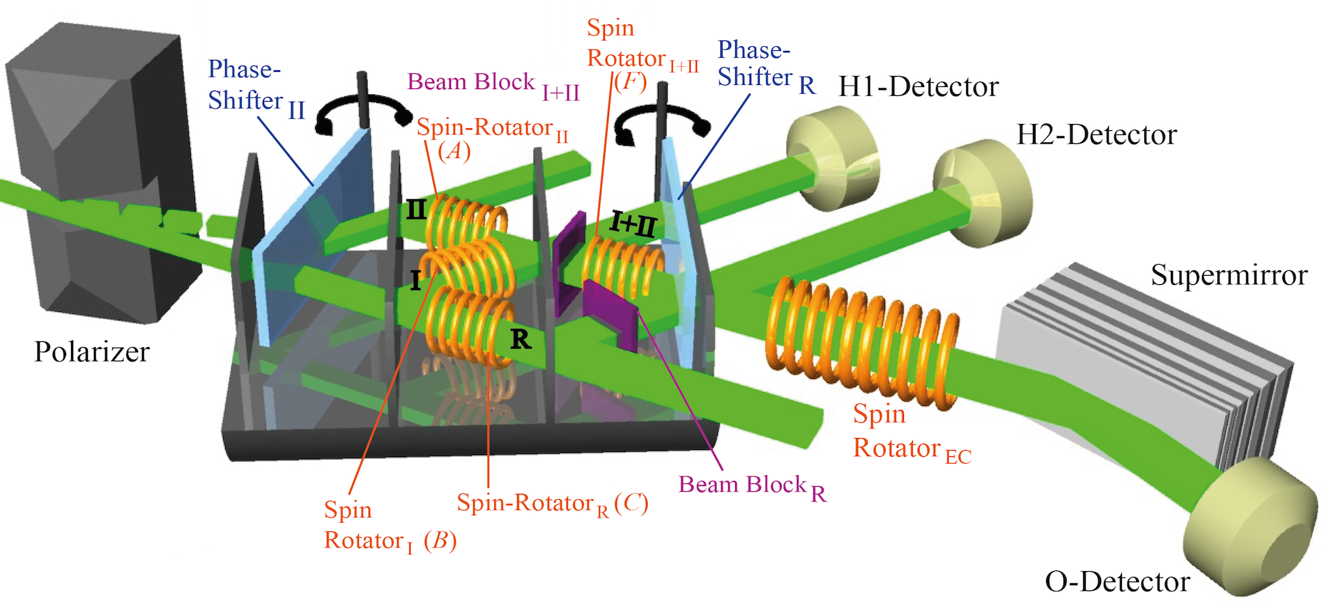 The IFM provides a conventional Mach-Zehnder like loop (front loop), which consists of two interfering beams in path and with  corresponding wave functions and . The two beams are recombined at the third plate of the IFM, yielding , where . The beam in forward direction in path is combined at the fourth plate of the IFM with the reference beam in path , with the wave function . The wave function in path O leaving the IFM in forward direction is given by . See below for a photography of the actual setup.

 The which-way (WW) measurement is achieved by applying resonance-frequency (RF) spin rotators (instead of vibrating mirrors as an Danan et al.). The neutrons in respective paths I, II, and R are marked by slightly shifting the energy by . The amount of which way marking is controlled by the rotation angle  of the neutron’s spins (see here for detailed calculations of the neutron’s wave functions and observed intensities).  The individual pathes are marked at different frequencies = 74 kHz, = 77 kHz, = 80 kHz, and = 71 kHz, respectively. All rotation angles used in the WW-marking =/9. Note that the wave functions before and after these spin rotators are still overlapping by 0.98, which justifies the condition of minimal perturbation due to WW marking. The energy compensating is set to the frequency = 68kHz. Next the intensity difference is calculated, where the stationary part cancel out and the time-modulating element emerges explicitly. The final, observed intensities in the detector is given by , consisting of the (stationary) intensity from the energy-unchanged main component  and the time-modulating one from the individual cross terms between the main component and the ww-marking components .

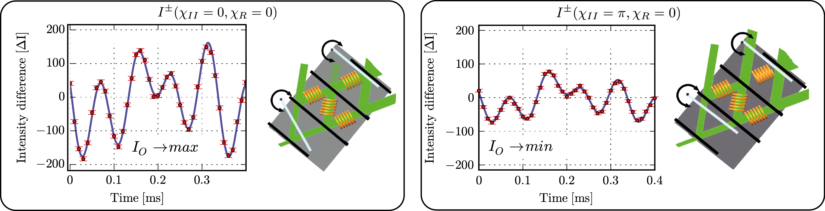
The time spectra , which are plotted above, are Fourier-analyzed in a standard manner using zero-padding and a Hanning windowing function. The obtained power spectra, together with a simulation with ideal circumstances (for instance full contrast of all interferometer loops), are depicted below. First we adjust the phase setting to , which is depicted below in the left panel of the interference measurements. We find all peaks at the expected frequency differences, namely kHz, kHz, kHz, and kHz. The ideal simulation, and the measurement have the same peak heights for the respective frequencies. The frequencies , , and are the same height, while is twice the height (the WW-signal from SR has to pass one beam splitter less than the other signals the way to the detector). Second, we adjust the phase setting , which is shown in the right panel of the interference measurements. Now two peculiarities are expected for the ideal simulation. (1.) The signal of SR is zero (no peak at ). (2.) The peaks at frequencies , and drop to one third, since the amplitude of becomes 1/3. Note that this behavior is predicated when simply calculating cross-terms in the formula of the intensity . The reason why we still observe this peak is due to imperfect destructive-interference in our interferometer. We observe a leakage of neutrons (in the main component) from the front loop to the beam path I+II.

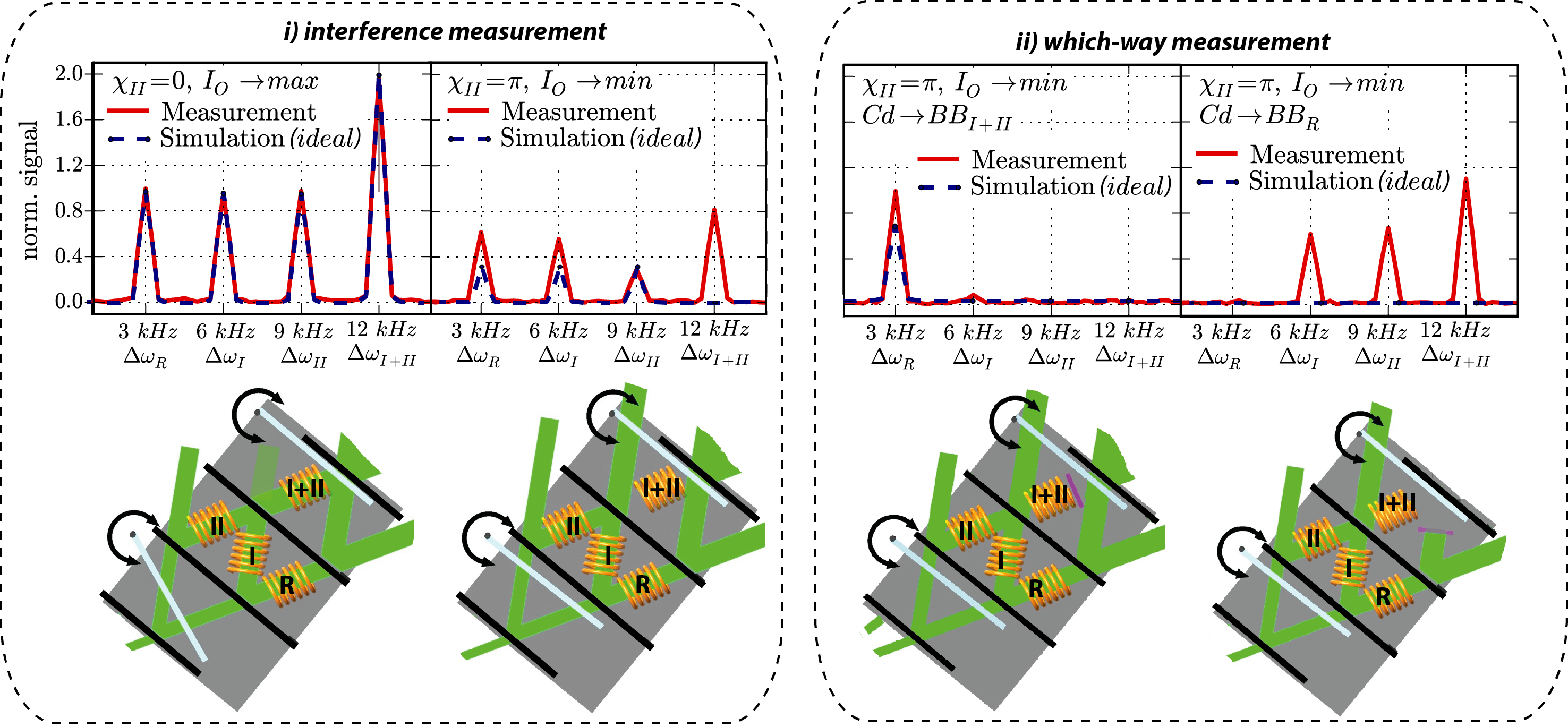
Placing a beab blocker (1mm cadmium slab) in the position BB (left plot of which-way measurement above), the beam in path R no longer contributes and therefore under ideal circumstances no peak at all are expected. this is so because , the mean intensity  and all cross-terms become zero (the peak at frequency vanishes since all components in path R are blocked). Finally, the beam-blocker is put in the position (right plot of which-way measurement above), where the WW-signals of SR, SR, and SR are blocked and the respective peaks are invisible in the power spectrum (lower row). In our measurement, due to leakage from the front loop, meaning contrast of is the main source for the occurrence of peak in principle no peaks should be observed.

Our  experiment confirms that standard quantum mechanics does provide an intuitive picture as well as a correct quantitative argument of the observed phenomena in the three-beam interferometer. Refuting the claim of Danan et al. that by the use of the two-state vector formulation a more intuitive understanding can be gained. Furthermore, in studying the interference effect, particularly in a destructive case, the occurrence of zero intensity is explained. This situation is interpreted in a mistaken manner as non-continuous trajectories in the paper of Danan et al.  Our results explicitly demonstrate that the sinusoidally-oscillating intensities, from which WW-information is derived, are attributed to the cross terms between the main energy-unshifted component and the WW-signals as predicted by a treatment in the framework of standard quantum mechanics.

1. A. Danan, D. Farfurnik, S. Bar-Ad, and L. Vaidman, Phys. Rev. Lett. 111, 240402 (2013). ↩

2. Y. Aharonov, P. G. Bergmann, and J. L. Lebowitz, Phys. Rev.  134, B1410 (1964). ↩

3. Hermann Geppert-Kleinrath, Tobias Denkmayr, Stephan Sponar, Hartmut Lemmel, Tobias Jenke, and Yuji Hasegawa, Phys. Rev. A  97, 052111 (2018). ↩