Geometric Phases

Evolving quantum systems acquire two kinds of phase factors: (i) the dynamical phase which depends on the dynamical properties of the system—like energy or time—during a particular evolution and (ii) the geometric phase which only depends on the path the system takes in state space on its way from the initial to the final state. Since its discovery by Shivaramakrishnan Pancharatnam and Sir Micheal V. Berry, the concept was widely expanded and has undergone several generalizations. Nonadiabatic and noncyclic evolutions as well as the off-diagonal case, where initial and final states are mutually orthogonal, have been considered.

Contents:

Berry’s phase – classic analogue
Berry’s phase – an adiabatic, cyclic evolution of a quantum system
””””Example – Neutron in a magnetic field
The geometric phase of Aharonov and Anandan – Nonadiabatic, cyclic evolution

Berry’s phase – a classic analogue

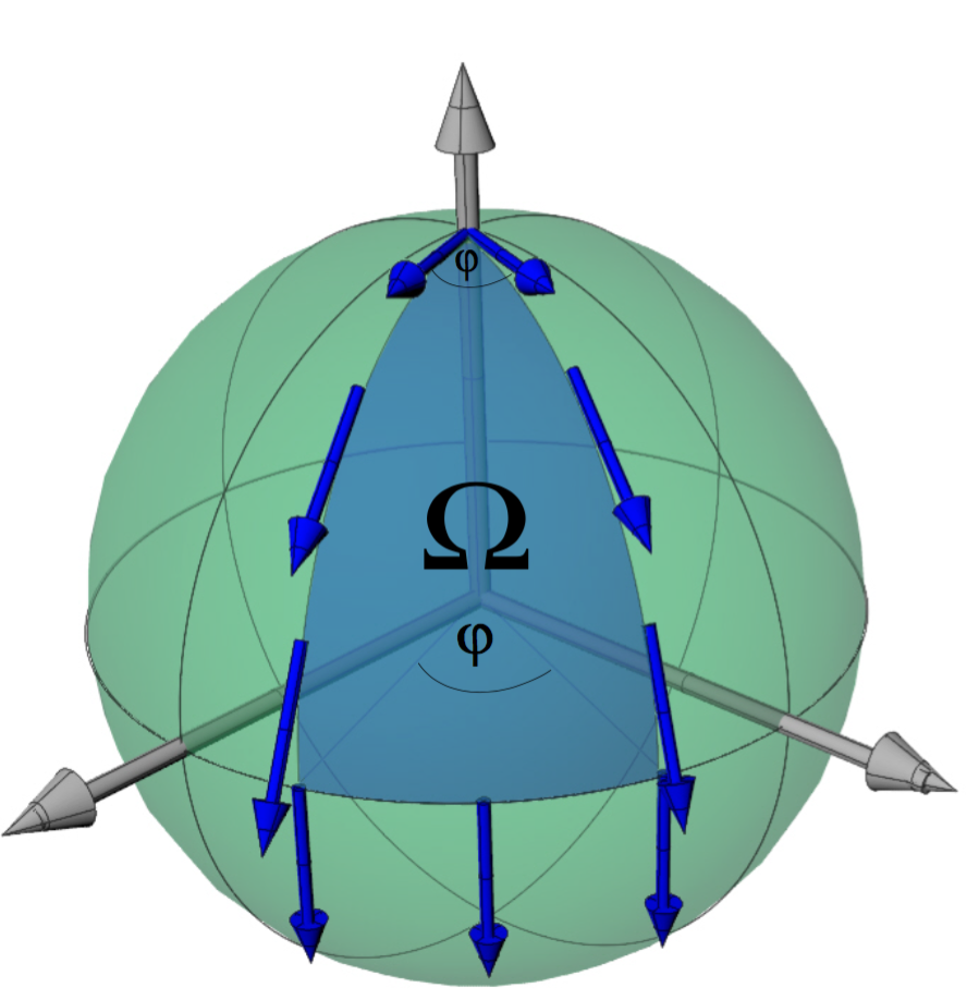
For understanding the concept of topological or geometric phases it is instructive to study an analogue from elementary geometry first. A vector pointing to an arbitrary direction is placed on the surface of a sphere. Now this vector is transported along a geodesic to the equator, along the equator and finally back to the starting point. During this transport the vector has to stay tangential to the surface. It does not change its magnitude and the angle between the vector and the geodesic path is kept constant at any time. If all these conditions are fulfilled during the whole process the transport is called parallel transport, which is depicted below. After finishing the excursion the vector has changed its direction by an angle . This angle equals the solid angle enclosed by the loop , since is the solid angle of a half-sphere and  is the portion surrounded by the loop.

Parallel transport of a vector on a sphere

Berry’s phase – an adiabatic, cyclic evolution of a quantum system

In 1984 Sir Micheal V. Berry published a paper ¹ in which he described the phase acquired by transporting a quantal system governed by the Hamiltonian depending on the parameters . The parameters change slowly, which means that adiabatic transformation is assumed. Consequently the system will remain in eigenstates of at any time . For a cyclic evolution the Hamiltonian takes on its original form at the final time and the system returns to its initial state. Thereby the state has been transported around a loop in parameter space, which is depicted below. Here is denoting the instantaneous state of the system, which is equivalent to the eigenstate . The time evolution of the system is given by the Schrödinger equation  . An eigenstate of at time is given by . A solution at time therefore is denoted as , with as an eigenstate of with energy . To calculate we have to insert this solution into the Schrödinger equation from above, which yields , multiplied by from the left side one gets . A solution can be found by integrating this equation , and applying the chain rule , which finally leads to , for a closed path in the parameter space with , which is depicted below. The first term corresponds to the usual expression of the phase accumulated by a system in a state with energy for a time , and is referred to as dynamical phase . The geometric phase is defined by the second term given by .

Example – Neutron in a magnetic field

Considering a system consisting of a neutron in a magnetic field with a Hamiltonian for the interaction between the spin an magnetic field is denoted as , where is the spin operator with the components of identified with the parameter . An arbitrary spin state can be parameterized in terms of the polar and azimuthal angle and , respectively: In the simplest case is static and direction of themagnetic field defines the quantisation axis, thus the Hamiltonian is given by . The time evolution of a neutron, initially in the eigenstate , according to the Schrödinger equation is denoted as . We get , where the Larmor frequency is . Thus the final state at is , where the phase factor denotes the dynamical phase proportional to the Zeeman energy. Since there is no evolution path in parameter space, caused by the Hamiltonian, there is no geometric phase.

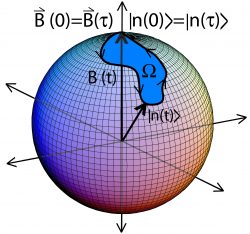
Curve traced out on  Bloch sphere

A completely different situation arises for a slowly changing of the Hamiltonian, assuming an adiabatic evolution. Here the neutron spin direction will be pinned to the direction of the magnetic field at any time, thereby remaining in an eigenstate of the Hamiltonian. Thus the state will acquire in addition a geometric (Berry) phase , which is independent of the Larmor frequency . The magnetic field is parameterized by the direction spherical coordinates and , respectively: with The corresponding eigenstates of the Hamiltonian are given by and . In order to derive the geometric phase associated to the spin-up state we have to calculate , where is given by with and . When an evolution along a circle of latitude was chosen, which yields a constant . Finally Berry’s phase is obtained by integration . For example if , a walk along the equatorial line, Berry’s phase is obtained as , which is minus half of the solid angle () as seen from the origin. For a longitude (geodesic) evolution along one always finds . As long as the magnetic field changes slowly, the system will remain in an eigenstate for all times and the geometric and dynamical phase components are given by and , respectively.

The geometric phase of Aharonov and Anandan – Nonadiabatic, cyclic evolution

In 1987, Berry’s phase was generalized by Yakir Aharonov and Jeeva Anandan ². They extended Berry’s result for a special case in the adiabatic approximation, to non-adiabatic and any cyclic evolution of a quantum system (for example a spinning particle in a static magnetic field). The key idea of this new concept is to associate the geometric phase with the closed curve in the projective Hilbert space instead of the parameter space of the Hamiltonian. Therefore the projective Hilbert or ray space has to be introduced: It is a general property of quantum-mechanical states that they are only defined modulo a phase factor, having no physical relevance. All states that differ merely by a phase factor give rise to the same physics. One might think at the first moment that discussions about the geometric phase are insignificant from this point of view, but a relative phase difference between two states in superposition, such as results in a different state. Only global phases can be neglected, for example and are indistinguishable. Assume a system evolves in a cyclic evolution, after one cycle the system is described as  with  real. The curve traced out in Hilbert space has an image in the projective Hilbert space as depicted below. Mathematically the projective space is defined over a projective map , where is a nonvanishing complex number}.

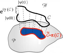
Projective Hilbert space (ray space) with an open curve C in Hilbert space

So the projective Hilbert space is a space in which an element is an equivalence class of state vectors that differ by multiplication by a nonvanishing complex number. Hence, now one can add additional phases at any point along the curve without changing the curve in projective Hilbert space. Suppose a state is given by with . Then and the Schrödinger equation becomes . The projections in of the curves traced out by and are the same (such as aninfinite number of other curves). However, the particular choice for has the advantage that the final phase difference can be split into a dynamical and a geometrical part as before. Integration results in , where the dynamical part is given by the first term , and the geometric phase arises from the second term and can be written as .

Since there are many curves projecting on to the same and one can find the same for all these Hamiltonians (due to an appropriate choice if ) the phase factor is independent of . So it does not depend on the choice of Hilbert space representation. Furthermore is independent of the choice of the parameter (reparametrisation invariance) and is uniquely defined up to , where is an integer: Considering two curves and with the same traced out by the state vectors and respectively with , where . They have the same geometric phase factor due to , which finally gives . Therefore all curves in that project to the same closed curve in have the same geometric phase modulo .

1. M. V. Berry Proc. R. Soc. Lond. A 391, 45 (1984). ↩

2. Y. Aharonov and J. Anandan Phys. Rev. Lett. A 58, 1593 (1987). ↩