Bell-type Inequalities and Local Hidden Variable Theories
October 11, 2016 5:27 pmAlbert Einstein , Boris Podolsky and Nathan Rosen (EPR) argued, based on the assumption of local realism, that quantum mechanics (QM) is not a complete. In 1951 David Bohm reformulated the EPR argument for spin observables of two spatially separated entangled particles to illuminate the essential features of the EPR paradox. Thereafter John S. Bell introduced inequalities for certain correlations which hold for the predictions of any local hidden variable theory (LHVT) applied, but are violated by QM. From this, one can conclude that QM cannot be reproduced by LHVTs.
Contents:
Bell’s theorm
Hidden variables formalism
Bell’s original inequality
The Clauser-Horne-Shimony-Holt (CHSH) Bell inequality
The spooky action at a distance or spukhafte Fernwirkung, as it was called originally by Albert Einstein in his correspondence with various physicists, can be explained if the measurement outcome is already pre-determined at the time of the states creation. However, this information is not part of the quantum-mechanical description, especially according to the Copenhagen interpretation of quantum mechanics, which at its very heart states that physical systems generally do not have definite properties prior to being measured, and quantum mechanics can only predict the probabilities that measurements will produce certain results – it is the effect of the measurement itself, that forces the system to reduce to only one of the possible values immediately after being measured. The Einstein–Podolsky–Rosen (EPR) paradox of 1935 is Albert Einsteins (and his colleagues Boris Podolsky and Nathan Rosen) attempt to demonstrate that the wave function does not provide a complete description of physical reality, and hence that the Copenhagen interpretation is unsatisfactory, or in their word incomplete (see here for details on the EPR thought experiment).
These are the two major assumptions of the EPR claim, namely reality and locality (or just local realism) summarized as it was done in the original paper:
Physical reality: Properties of physical systems are those physical quantities whose value can be predicted with certainty before carrying out the corresponding measurement. These properties are in reality already determined before they are measured. They are elements of reality. This concept is called Einstein reality:”If without in any way disturbing the system, we can predict with certainty the value of a physical quantity, the there exists an element of reality corresponding to this physical quantity”1. This means that this physical quantity has a value independent of weather it is measured or not.
Locality: Physical reality can described locally. Meaning that the properties of a physical system (i.e. the value of a measurement) is independent of which interventions (measurements) are carried out on an other spatially separated system. This concept is called Einstein locality;”The real factual situation of a system A is independent of what is done with system B, which is spatially separated from the former.”1
The authors of the EPR paper argued based on local realism that quantum mechanics is not structured finely enough to capture all the elements of the physical reality (which are always present, weater measured or not). They concluded from this assumption that quantum mechanics is not incorrect but incomplete. There are elements of reality that do not appear in quantum theory, and therefore they are hidden variables for quantum theory.
Bell’s theorm
In his groundbreaking paper, published in 1964 paper, entitled ”On the Einstein Podolsky Rosen paradox” 2, Northern Irish physicist John Stewart Bell presented an analogy, based on spin measurements on pairs of entangled electrons, to EPR’s hypothetical paradox. In its simplest form, Bell’s theorem can be formulated as follows: No physical theory based on the joint assumption of locality and realism can ever reproduce all of the predictions of quantum mechanics. The source of Bell’s interest in non-locality was his detailed analysis of the problem of hidden variables in quantum theory and in particular his studies of the Broglie–Bohm “pilot-wave” theory, which is nowadays usually referred to as Bohemian mechanics 3.
Hidden variables formalism:
A set of supplementary parameters, i.e,. hidden variables, denoted represents all elements of reality which occur in connection with a polarization measurement. All properties of an object are characterized by a certain set of variables . Particles with values of the variables are emitted by a source with a probability with for . The only possible outcomes of a polarization measurement at A for an angle of rotation of the analyzer are +1 or -1. Then there exists an unambiguous function , which for a given and determines the measurement value definitely as +1 or -1, which are the only two possible results of . The same is valid for the polarization measurement at B along . A particular hidden variable theory is completely defined by the explicit form of the functions , and . In a next step the probabilities of the various measurements results can be calculated via the function , which gives +1 for the +(1) result, and 0 for the -(1) result. In the same applies for assumes the value +1 for the -(1) result, and 0 otherwise. Thus the probability to measure +1 at polarizer A, at the angle α is given by . The joint probability to measure +1 at polarizer A, at the angle and -1 at polarizer B at the angle is .The classical correlation function is then expressed as . The fact that the correlation is given by a product of the two functions and expresses locality. So the result of does not depend on the measurement settings at B, and vice versa.
A naive example: At this point it is informative to introduce a simple example of supplementary parameters theory, where each photon pair is supposed to have a well defined linear polarization, determined by its angle with the x-axis at sides A and B, as illustrated below.

To account for the strong correlation the two photons of a same pair are emitted with the same linear polarization, defined by the common angle . The polarization of the various pairs should be randomly distributed, consequently the probability distribution is assumed to be rotationally invariant expressed as . To complete this model explicit forms of the functions and have to be defined such as and . is assigned the value +1 when the polarization of photon encloses an angle less than with the direction of analysis and -1 for the complementary case, where the polarization is closer to the perpendicular to . With this explicit model the various probabilities of the polarization measurements can be compared with the predictions of quantum mechanics: . These results are identical to the quantum-mechanical results for the entangled state , where and denote the polarization’s along and -direction, respectively. Using projection operators given by and where and , gives the following probabilities for single measurements , which means that individual polarization measurement gives a random result – a typical quantum property !
For joint probabilities, or equivalently the correlation function, we get , for , which is plotted on the right side. However, now the predictions of quantum mechanics are different: Considering the probabilities for joint detection we get

So the probability of finding both photons in the same polarization is given by and the probability of finding both photons in the different polarization is . A method to measure the amount of correlations between random quantities, is to calculate the correlation coefficient. For the polarization measurements it is equal to . To sum up, the quantum-mechanical calculations show that although each individual measurement gives a random result, these random results are correlated and for parallel analyzers full anti-correlation is observed. At this point we want to emphasize, that for spin- particles in an entangled state the projection operators onto an arbitrary spin direction are given by with and , which yields . So for spin -particles the angles are typically half as large compared to photons. While our naive example of supplementary parameters theory does not completely reproduce the predictions of quantum mechanics it is a remarkable result! First depends only on the relative angle between and , such as the predictions of quantum mechanics. Second, the difference between the predictions of this simple supplementary parameters model and the quantum-mechanical predictions is always small. This could suggest that a more sophisticated model could be able to reproduce exactly the quantum-mechanical predictions. But this is not the case! Bell’s discovery was the fact that the search for such local realistic models is hopeless, as will we demonstrated next !
Bell’s original inequality:
According to quantum theory, when spin measurements along different axes are performed on the pair of particles (labeled particle 1 and particle 2) in the singlet state, , the probability that the two results will be opposite is given by , where is the angle between the chosen axes. Now we consider three particular axes and , lying in a single plane and are such that the angle between any two of them is equal to . Since , an agreement with the predictions of quantum mechanics is found if if , with being the probability of the pre-determined outcome of the spin measurement for particles 1 and 2 (assuming only two possible values, say 1 for “up” and -1 for “down”) of the variable . However, agreement with the predictions of quantum mechanics in addition requires opposite outcomes for identical measurement axes, namely , for arbitrary values of . But it turns out that it is impossible to satisfy both requirements, which is referred to as Bell’s inequality theorem.
Under the assumption of pre-defined values, the 8 possible particle types (including their pre-defined spin values along directions and are listed in the following table:
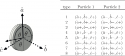
Assuming that all 8 particle types occur with the same probability can be treated mathematically as a random variable we get Eq.(i): . This can simply be checked by counting the respective frequencies of occurrence in the table, which gives , verifying Bell’s inequality theorem. Proof: The three ±1-valued random variables can’t all disagree, from which immediately follows that , but since we have , proving Bell’s inequality theorem.
However, according to quantum mechanics each term on the left-hand side of the equation describing Bell’s inequality theorem gives , which in total yields , establishing the incompatibility between the quantum predictions and a possible existence of pre-existing values.
In his original paper 2 Bell expressed his inequality in terms of correlation functions instead of probabilities of the disagreement Eq.(ii): . These formulations are nevertheless equal since the correlation function is defined as the expected value of the product , which reads . This in turn can be rewritten as . Now we can rewrite inequality Eq.(i) in terms of the correlations obtaining , because of the perfect anti-correlations we finally get . From this Bell’s original inequality Eq.(ii) follows from the conjunction of two inequalities (due to the absolute value). One is obtained by changing the signs of and ant the other one by hanging the signs of and again .
The Clauser-Horne-Shimony-Holt (CHSH) Bell inequality: Bell’s theorem without perfect correlations
Since perfect correlations are only very hard to achieve in an actual experiment Bell’s original inequality, while extremely simple, is not suited for an experimental test. In 1969 John Clauser, Michael Horne, Abner Shimony, and Richard Holt (CHSH) reformulated Bell’s inequalities pertinent for the first practical test of quantum non-locality, applying a slightly more complicate arrangement of measurement settings: At analyzer A measurements are carried out with the orientations and and at B with and accordingly. Assuming local realism all four measurements have predefined values denoted as and which can only take the values +1 or -1. The identity holds for any random set of the four values. By accumulating data one can average the four terms and construct the algebraic sum of a quantity which can take only the values ±2. Hence, the sum must be bounded within these limits:
On the other hand quantum mechanics predicts for the expectation value . Hence the algebraic sum can be written as . As shown in figure below (left) of the CHSH inequality the relative angles between the measurement directions are given by and
, which leads to . A maximal violation of the CHSH-Bell inequality is found for , for spin-1/2particles, which corresponds to for photons, where , which is illustrated in the plot below (right). A value of is found at for spin-1/2 particles (photons correspondingly ).

(left) CHSH measurement directions. (right) S value for Spin 1/2 particles and photons.
Let us see in more detail, considering a function with only possible values expressed as :


Using the classical correlation coefficients from the hidden variables formalism, introduced above, one finally obtains . However, quantum mechanics predicts for the corresponding measurement on correlated spins, with angles , , and (again for photons half of these angles). and . Hence, in total we get , which is greater than 2, and CHSH violations are therefore predicted by the theory of quantum mechanics.
1. A. Einstein, B. Podolsky, and N. Rosen, Phys. Rev. 47, 777 (1935). ↩
2. J.S. Bell Phys. Rev. 1, 195-200 (1964). ↩
3. S. Goldstein, Bohmian mechanics, The Stanford Encyclopedia of Philosophy (2001, revised in 2006). ↩