Tight qubit uncertainty relations

September 28, 2026 3:07 pm Published by Stephan Sponar

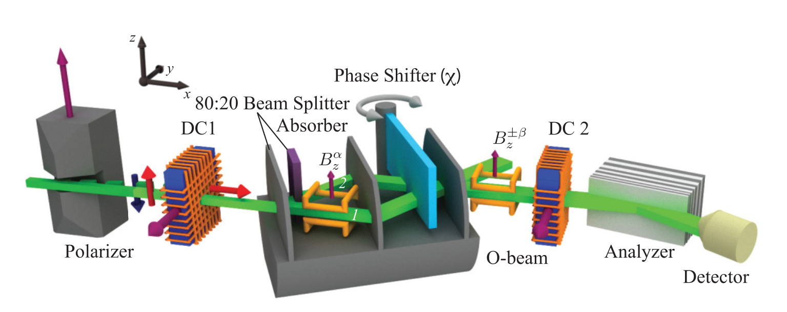
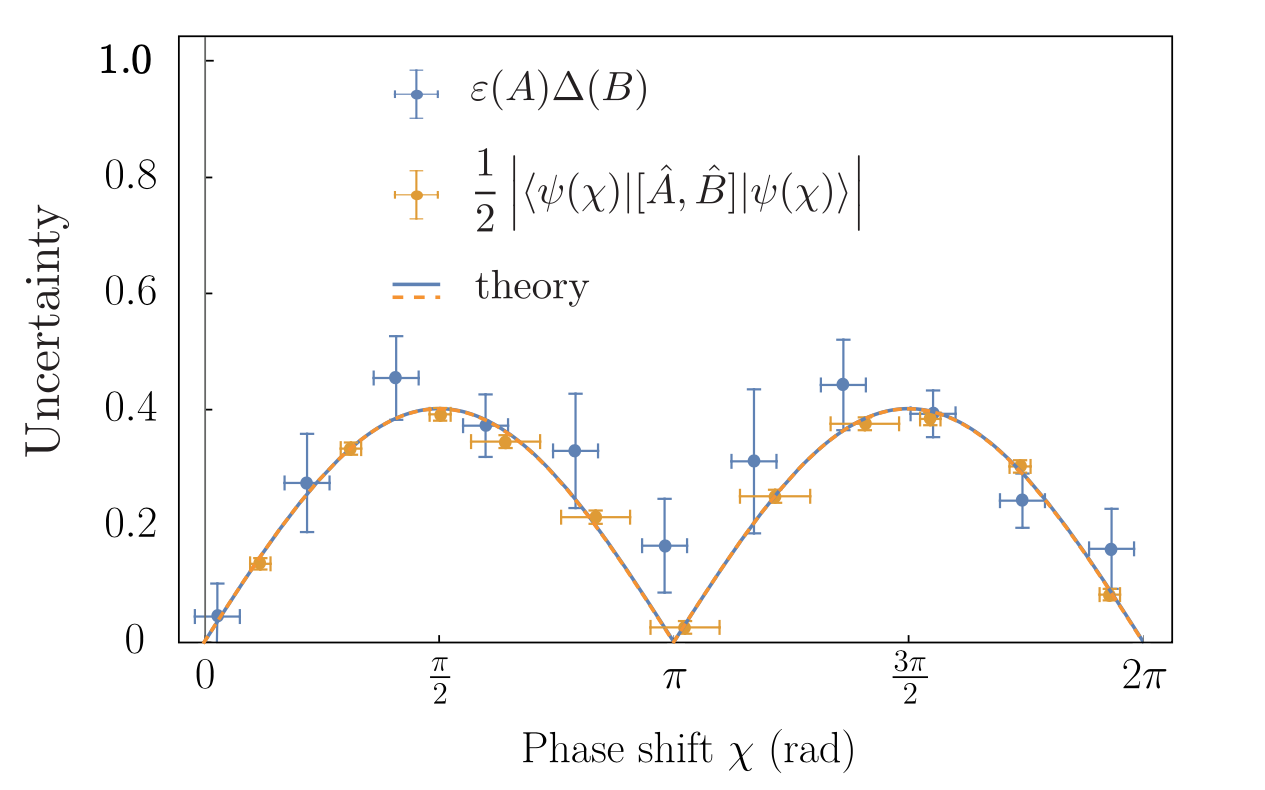
In our latest interferometric experiment ¹ we compare measurements of the Ozawa-Hall error and the measured lower bound of Ozawa’s universally valid uncertainty relations as function of initial states’s phase for observables and . The former is a which-way observable in an interferometer, while the latter observable is associated with the output of the interferometer. Since the first observable is measured in a non-invasive manner, applying the so-called feedback compensation (see ²for details), the measurement of the second observable is not disturbed. This results in a tight version of Ozawa’s universally valid uncertainty relation, denoted as , where we experimentally verify both sides of the (in)equality, applying the setup depicted below.

1. Core Theoretical Framework & Mathematical Formulations

Heisenberg’s original formulation of the error-disturbance trade-off fails under certain measurement conditions. Masanao Ozawa derived a universally valid relation, which was subsequently given a statistical interpretation by Michael J. W. Hall using quantum weak values.

Ozawa’s Universally Valid Uncertainty Relation (Linear Form)

Ozawa introduces state-dependent standard deviations to ensure the inequality holds true for all arbitrary states and measurement devices, employing a linear term matrix:

ε(A)η(B) + ε(A)σ(B) + σ(A)η(B) ≥ ½ |⟨[A, B]⟩|

Where:

ε(A) is the measurement root-mean-square (rms) error of observable A.
η(B) is the physical disturbance induced on a conjugate observable B.
σ(A) and σ(B) represent the intrinsic quantum standard deviations of the operators calculated on the initial state |ψ⟩.

e root-mean-square error ε(A) reaches exactly zero.

3. Final Structural Synthesis

Statistical Deviation and Complex Weak Values

Hall’s framework equates measurement error to the statistical divergence from an optimal estimate. The optimal estimate of an operator A given a pre-selected state |ψ⟩ and a final post-selected state |m⟩ corresponds exactly to the real part of the quantum weak value:

⟨A⟩_w(m) = ⟨m|A|ψ⟩ / ⟨m|ψ⟩

Because the experimental estimator must be purely real while the weak value can be complex, the squared error breaks down analytically via the Pythagorean theorem:

ε(A)² = ∑_m p(m) [ (a(m) – Re⟨A⟩_w(m))² + (Im⟨A⟩_w(m))² ]

This formulation yields a fundamental quantum insight: even with a flawless classical estimator where a(m) = Re⟨A⟩_w(m), the error cannot vanish unless the imaginary component of the weak value is zero (Im⟨A⟩_w = 0). The imaginary part represents the unavoidable back-action noise of quantum mechanics.

Branciard’s Tight Boundary Extension (Squared Domain)

In this experimental architecture, the disturbance on the conjugate observable is zero (η(B) = 0). Under this restriction, Ozawa’s relation reduces to the much tighter, squared Branciard boundary:

ε(A)² σ(B)² ≥ ¼ |⟨[A, B]⟩|²

The paper proves that for pure quantum states, this inequality saturates exactly at its lowest limit, indicating the relation is tightly fulfilled without mathematical slack.

2. The Neutron Optical Experiment

The experimental setup was conducted at the S18 instrument of the Institut Laue-Langevin (ILL) in Grenoble, France, utilizing a perfect-crystal silicon Mach-Zehnder neutron interferometer. Polarized monochromatic neutrons enter the interferometer and are split into paths |1⟩ and |2⟩ at the first interferometer plate at a ratio of 1 : 4. Before the interferometer, the probe qubit is prepared in the initial spin state |Sin ⟩ = |s↑x ⟩ by a π /2 direct-current spin rotator (DC 1). In path 1, the spin is rotated by an angle α. Beam stop and phase shifter are required for which-path or interference measurements, respectively. Behind the interferometer, the compensation is applied, that is, a spin rotation by angle β±, dependent of the respective measurement context. The spin is analyzed in ±x direction by the combination of a π/2 direct-current spin rotator (DC 2) and the magnetic supermirror. The neutrons are counted in a 3He detector.

Physical Mapping of the Qubit

A monochromatic neutron beam enters the interferometer and is split into two spatially separated paths, Path I and Path II, by a silicon crystal plate. The qubit system under examination is mapped natively onto these two degrees of freedom:

The system state is represented by the path presence of the neutron inside the interferometer.
The internal neutron spin state serves as the meter (probe system) that records information about the path.

The Implementation of Feedback Compensation

To extract the real parts of complex weak values without destroying the quantum system through strong measurements, the authors applied an innovative feedback compensation technique:

Weak Coupling: A small spin-rotation angle α is introduced in one of the paths via a localized magnetic field. This establishes a weak coupling between the path presence (system) and the spin (probe).
Compensation: Rather than performing tomographic reconstruction, a feedback spin rotation β is introduced right before the final beam recombination.
Extraction: By fine-tuning β until the induced weak decoherence shifts are perfectly balanced out (nullified geometric phase shift), the real part of the complex weak value is directly read out from the physical angle of the control element.

By scanning the relative phase between the interferometer paths, the team cleanly isolated the dependencies of Re⟨A⟩_w and Im⟨A⟩_w, validating that when the system phase causes the imaginary part to transition through zero, the root-mean-square error ε(A) reaches exactly zero.

3. Structural Synthesis

Parameter / Framework	Theoretical Component & Formula	Experimental Realization (Neutron Optics)
Quantum System Setup	Qubit Space: `\|ψ⟩` and `\|m⟩`	Perfect-crystal Mach-Zehnder setup splitting neutrons into Path I and Path II.
Quantum Probe (Meter)	Meter Operator: `M = ∑ m P_M(m)`	Neutron spin state manipulated by localized magnetic fields.
Error Tracking Mechanics	`ε(A)² ~ (Im⟨A⟩_w(m))²`	Feedback compensation: Translating weak shifts into measurable spin rotation control angles (α, β).
Boundary Tightness	Branciard Inequality: `ε(A)² σ(B)² ≥ ¼ \|⟨[A, B]⟩\|²`	Pure state operation confirms that the relation saturates exactly at its lowest limit.

4. Final Experimental Results

The measurement error vanishes completely for phase settings where the weak value is purely real (imaginary part is zero). Since the lower bound of the uncertainty relation is given by the gradient of the interference fringe the bound also vanishes at the same phases, namely and . This illustrates that in Ozawa’s theory of measurement errors the imaginary part of the weak value is associated with the error (see here for details of the experiment and more results). This work was supported by the Austrian science fund (FWF) Projects No. P 34239, P 30677, and P 34105.

1. Andreas Dvorak, Ismaele V. Masiello, Yuji Hasegawa, Hartmut Lemmel, Holger F. Hofmann, and Stephan Sponar, Phys. Rev. Res. 7, 043334 (2025). ↩

2. Hartmut Lemmel, Niels Geerits, Armin Danner, Holger F. Hofmann, and Stephan Sponar, Phs. Rev. Research 4, 023075 (2022). ↩